|
3D Geometry Primer: Chapter 1 - Issue 09 - Barycentric Combinations by (09 October 2000) |
Return to The Archives |
Barycentric Combinations
 |
| I promised it last week. Today we're going to examine barycentric combinations. What they are, how they are, why they are ... It's going to be *very* mathematical, so don't be too scared. (BTW: Freddy, if you read this by now: de groetjes wî!) |
(I) Linear Combinations Of Points (Still Dependent On The Origin)
 |
|
Like I already mentioned last week, barycentric combinations are special
linear combinations of points. Before we can examine what's so special
about them, we first have to take a better look at linear combinations
themselves. What's a linear combination of points? Let's say we want to take a linear combination of n points P[0], P[1], ... , P[n-1] and we call the result Q. 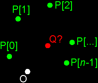 To calculate Q, you simply take the sum of all points P[0], ..., P[n-1] in which each point P[i] is scaled with a real factor. That factor is called the weight-factor of that point and is written as w[i]. The weight-factor w[i] of each point P[i] determines how much that point affects the sum. It tells you how much the point Q is influenced by the point P[i]. This all looks like this: Q = w[0]*P[0] + w[1]*P[1] + w[2]*P[2] + ... + w[i]*P[i] + ... + w[n-2]*P[n-2] + w[n-1]*P[n-1]. In maths, we abbreviate this as follows:  If you don't know what that weird S-symbol means, you should check out remark 1, because we're going to use it quite a lot this issue. If you don't feel comfortable with it, then you might write out each of these. It will help you to understand it. So, Q is the sum of P[0] to P[n-1] in which each P[i] has a weight factor w[i]. But now you ask: "What does it mean, that sum of points? How do you apply those weight-factors? You've never talked about *that*!" Well, I'm going to do this right now ... What does that sum mean? Well, you remember last issue, where I asked you to add 2 points together? You couldn't do that until I showed their place vectors. Then your instinct tried to add those place vectors together (at least, let's hope so). This was very logical, but unfortunately *wrong* because it depended on the origin. It still does, but later in this issue we'll see how to solve that problem by choosing the weight-factors very carefully. So, *for now*, to add those points P[0], ... , P[n-1] together, simply add their place vectors OP[0], ... , OP[n-1]. And then you become the place vector OQ of the resulting point Q. Don't worry if it depends on the origin, we'll solve that later. How do you apply those weight-factors? Now you know that we actually summon the place vectors (In other words: we take a linear combination of the place vectors), you should easily see that this multiplication of a real value w[i] and a point P[i] will be replaced by a simple scalar product w[i]*OP[i]. And we all know what that scalar product means: it scales the magnitude of the place vector. I'll give you here a little example to show you how easy it is. Say you have 3 points P[0], P[1] and P[2] (I didn't draw these points explicit in order to not overload the already overloaded picture, but as you know, these points are the heads of the 3 place vectors OP[0], OP[1] and OP[2]). Now you want to know the following linear combination of these points: Q = 3*P[0] + 2*P[1] + (1.5)*P[2]. How do we do that? 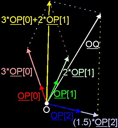 Well, as I've already said, the point Q is given by its place vector OQ which is found by exactly the same linear combination of the place vectors: OQ = 3*OP[0] + 2*OP[1] + (1.5)*OP[2]. To calculate this, you first construct the 3 scalar products 3*OP[0], 2*OP[1] and (1.5)*OP[2]. Then you add 2 of these scaled vectors together, e.g. 3*OP[0] + 2*OP[1] which give you the yellow vector. Then you add the 3rd vector to this sum which gives you the white vector OQ. I hope this is clear enough, otherwise you should try this on a sheet of paper. So, the linear combination of points has become a linear combination of vectors ... 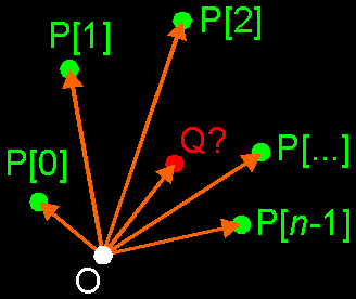  |
(II) Barycentric Combination (Not So Dependent Anymore)
 |
|
Now that we know how to do linear combinations of points, we want to find a way
to make this independent of the origin and to become the barycentric
combinations. We'll do this by putting conditions on the weight-factors
w[i]. Let's take another look at expression (9.1).  We already know that if we put this in the computer, we will actually use the expression (9.2a) since we'll use place vectors to store all points.  How can we find the condition in this? Well, I hope that you remember of last week that the difference of 2 points is a vector that fits in between those points. Now, each place vector, like OP[i] fits between the origin O and the point P[i]. So, we can write each place vector as the difference of the point in question and the origin: OP[i] = P[i] – O and OQ = Q – O. If we use this to replace each place vector in expression (9.2a), then we get this:  You might find it a bit weird to subtract the origin from a point, since the origin has coordinates O(0,0,0); but then you forget again that in the real world, the origin is just another point that has to be treated like all the others. So, ignore the fact that the origin is that special (0,0,0) for now. Since we have again a sum of points, we need to convert this to place vectors once again. Otherwise, we can't use our vector arithmetics on it. Last time we used our origin O to define all place vectors, but we have a problem now: this time we have to find the place vector of the origin O itself. Therefore we're going to choose a new origin for this one: O'. This doesn't change anything to the problem since our goal is to find a solution independent on the origin (or in other words, a solution that counts for every origin, and thus also for O'). So, we replace the point Q by O'Q, P[i] by O'P[i] and O by O'O.  Do this also for the original problem (9.1). Replace the points Q and P[i] by place vectors using the origin O'.  Compare this expression (9.2b) with (9.2a), and convince yourself of the fact that both expressions are equivalent translations of (9.1). This is of course, and again, because (9.1) has to be independent of the origin. Now, concentrate on the right term of expression (9.4). We see a summation of w[i]*(O'P[i] – O'O). Use the distributive property of vector arithmetic (this is: r*(U+V) = r*U + r*V) to write this as w[i]*O'P[i] – w[i]*O'O. You get the following expression:  Now, you can split up the summation into 2 different summations. Check out remark 1 if you don't follow in this.  You see that I've colored expression (9.6) in 2 different colors: red and green. Take a look at the green parts (ignore the red parts), and convince yourself that this is exactly the same as expression (9.2b). So, (9.6) can be seen as (9.2b) *plus* in each term the extra red parts. Now, we do know that (9.2b) and (9.6) must be equivalent since both expressions are just a "translation" of the original problem (9.1). (9.2b) and (9.6) can only be equivalent if the left red part and the right red part are equal. If you have 2 normal real equations a = b and a – c = b – d, then both both equation can only be equivalent if c = d. I hope you see that. Here, you can use the same reasoning to demand the following thing:  You can see that both terms are scalar products of the vector O'O (see the left one as 1*O'O). These products can only be equal if both scalars are equal:  Or in other words: the sum of all weight-factors w[i] must be 1. This is *the* condition to achieve the independency you need for the barycentric combination. You don't believe this? Well, you need *this* condition (9.8) to make sure that expressions (9.2a) and (9.2b) are equivalent: you can rewrite (9.2a) as (9.6) without it, but then you need (9.8) to rewrite (9.6) as (9.2b). Now, you can write the "formula" for barycentric combinations in one line:  You can remember this by the following ... Take a look at (9.2a): "To have the place vector OQ of Q at the left side, you need the origin O exactly 1 time. So, to make sure this is equal to the right side, you need the origin O exactly 1 time at the right side too. Thus the sum of the w[i]'s must be 1." You must see that there are many many ways to choose the w[i]'s so that their sum is 1. Then you can also see that there're many many possible barycentric combinations of one set P[i]'s. In fact, there are an infinite number of it. In that infinite set of barycentric combinations of those P[i]'s, there's one special subset: the convex barycentric combinations ... |
(III) Convex Barycentric Combinations & Convex Hull
 |
|
Definition: If all weight-factors w[i] are positive
(each w[i] ł 0), then you have a
convex barycentric combination. If you take – in the set of all possible
barycentric combinations of the points P[i] – the subset of all convex
barycentric combinations, then you have the convex hull. The convex hull is the smallest polygon or polyhedra (filled and convex), enclosing a set of points P[i]. I've said "polygon or polyhedra", why? Well, if these points P[i] are co-planar (i.e. they lay in the same plane), you will have a polygon as convex hull. If they are not, you will have a polyhedra. But if you see a polygon as a "flat polyhedra", then you can talk about the convex hull as a polyhedra only. You can find this polyhedra by "drawing" between each 3 different points of the set P[i] a triangle. There will be many triangles intersecting each other, but that doesn't matter. You only have to look to the outer triangles. They don't intersect any other triangle, and form a completely closed polyhedra: the convex hull. All other triangles will be inside that polyhedra. You can see that most faces of the convex hull will be triangles. Although these triangles can form "higher polygons" as faces, if they're co-planar. e.g. 2 co-planar triangles that share an edge, form 1 quadrangle. Now, it shouldn't be to hard to see that if the points P[i] are all co-planar, you will have a "flat polyhedra" and thus a polygon as convex hull. Notice that the convex hull exists of *both* the edge and the inner side of the polygon/polyhedra. In the case of co-planar points P[i], it's even more simple to find the convex hull. All you do, is to take an "elastic band" and to tighen it around the points P[i]. Then the band will take the shape of the convex hull automatically. I'll work further with these "flat" convex hulls, since it is easier to draw them. But everything I'll tell you about it, applies also on "non-flat" convex hulls. 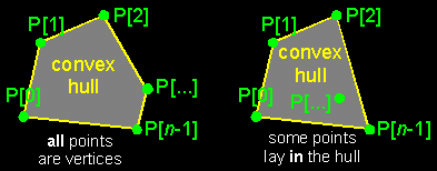 As you can see in the previous picture, the vertices of the convex hull are points of the set P[i]. But this doesn't work in the other way: not all of the points P[i] will be vertices (see right picture). Some of the points P[i] will be inside the convex hull. This is something to remember! If the points P[i] are already the vertices of a convex polygon, then it isn't to hard to see that the convex hull will be exactly the same of that original polygon. And also, if the original polygon isn't convex, then the convex hull be larger than it. (see next picture). 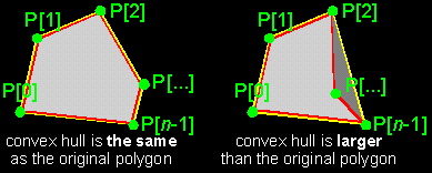 You can use this property if you need a point *inside* a convex polygon. All you have to do is to take a convex combination of the vertices. I'll show that in example (b). But don't forget that you need a *convex* polygon to do that! |
(IV) Examples ...
 |
|
a) MIDDLE OF 2 POINTS: You can find the middle Q of 2 points P[0] and P[1], by choosing your weight-factors w[0]=1/2 and w[1]=1/2: Q = (1/2)*P[0] + (1/2)*P[1] = (P[0] + P[1])/2. I guess you already knew that. But if you don't believe me, you should try this on a sheet of paper. Draw 2 points P[0], P[1] and a origin O. Draw the place vectors OP[0], OP[1] and construct OQ; you will see that this point Q will be indeed in the middle of P[0] and P[1]. Notice that this is also a convex barycentric combination. b) BARYCENTRE: If you have a set of n points P[0], P[1], ... , P[n-1], then choose your weight-factors as w[i]=1/n. Convince yourself that the sum of the weight-factors is 1 and that this is a convex barycentric combination. It's a combination in which each point is as important as the others, since they have all the same weight 1/n.  This special combination is called the *barycentre* and is in fact the "centre of mass" of the n equal mass points P[i]. You should check out a book about theoretical mechanics to know what that exactly means, but here, it's another property of the barycentre that is important: the barycentre lays *always* inside the convex hull. If the points P[i] are already the vertices of a convex polygon/hedra, then the barycentre will lay *inside* that polygon/hedra, since that polygon/hedra is exactly the convex hull. If you have e.g. an triangle, a pyramid, a square, a cube, or any other (convex!) polygon or -hedra, then you know that the barycentre of the vertices lays inside that thing. Use that if you need such a point!  Notice that example (a) is nothing more than the barycentre of 2 points. c) LINES: We know that through 2 different points A and B goes exactly 1 line AB! And that line is of course independent of any origin. In the next chapter we'll see that the parameter representation of that line is: P = (1–t)*A + t*B. If you take all t's between –Ą and +Ą, then you get all the points P of that line. You can see that P is for each t a barycentric combination since t + (1–t) = 1. This makes it independent of the origin. If you make sure that (1–t) ł 0 and t ł 0, then you get only the convex combinations which lay exactly between A and B, then you get only the points of line segment [AB]. To achieve this, you must take t between 0 and 1: 0 Ł t Ł 1. d) PLANES: We know that through 3 different, non-linear points A, B and C goes exactly 1 plane ABC! And that plane is of course independent of any origin. In the next chapter we'll see that the parameter representation of that plane is: P = (1–u–v)*A + u*B + v*C. If you take all u's and v's between –Ą and +Ą, then you get all the points P of that plane. You can see that P is for each u and v a barycentric combination since (1–u–v) + u + v = 1. This makes it independent of the origin. If you make sure that (1–u–v) ł 0, u ł 0 and v ł 0, then you get only the convex combinations which lay exactly between A, B and C, then you get only the points of triangle ABC. To achieve this, you must take e.g. u between 0 and 1 and v between 0 and (1–u): 0 Ł u Ł 1 and 0 Ł v Ł (1–u). e) BEZIER, B-SPLINE, ... All these special curves and surfaces use barycentric combinations to make sure that their result is independent of the origin, just like a line or plane is. I can't go further on that, but if you read a tutorial on one of these, keep that in mind. Maybe we'll come back on this in one or other chapter that follows. |
(V) Bramz Says "GoodNight Folks!"
 |
|
This is it. We have finished chapter I. Now you know how to deal with vectors
and points in any dimension, and what their relationship is. Maybe there will
be an addendum next week with some examples and things I've forgotten to tell
you, but then this chapter will be finally over. This means that it's time now, to think about chapter II. It will handle the basic primitives of 3D space: lines, planes, spheres and maybe cilindres and cones. It can take a few weeks/months till things are set up, but then we'll continue with the 3D Geometry Primer. So don't worry if you don't hear anything from me. I hope you'll be staying up so long, 'cause I will. the Bramz. "There are 3 kind of mathematicians: those who can count and those who can't" |
Remarks
 |
|
(1) That weird S-symbol is the Greek letter Sigma and
is called the summation symbol. It provides you a way to abbreviate many sums.
First, I'll give you the equivalent of it in pseudo-code and C. The following expression ...  ... is in pseudo-code ... sum ¬ 0; for each i from min to max sum ¬ sum + something[i]; next i ... and in C ... sum = 0; for (i = min; i <= max; i++) sum += something[i]; I'll give you a little example here:  It is very helpful to write out such a summation this way, if you don't feel comfortable with it. It gives you a better idea of how it works. I have to tell you one more thing about this kind of summations (there's much more to tell about this, but it will be all you need for today). It's a way to split up one summation in 2 summations. Follow this: 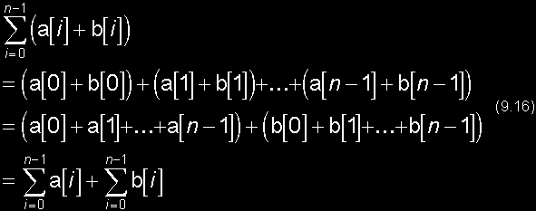 In the first line, you have "under the S-symbol" (that's how we refer to the stuff that is summoned) another little sum a[i] + b[i]. If you write this out (2nd line) and you carefully rearrange all terms (3rd line); then you can finally rewrite this as a sum of 2 summations: one of the a[i]'s and one of the b[i]'s (4th line). This is what we'll do to step from (9.5) to (9.6). |