|
Raytracing Topics & Techniques - Part 5: Soft Shadows by (05 November 2004) |
Return to The Archives |
Introduction
 |
|
It's time to do something useful with the new speed that the regular grid brought us. Ray tracing speed is just like money: You always spend twice the amount you actually have. :) One of the finest things to spend it on is soft shadows. They are reasonably easy to do, so this article will be a bit lighter than the previous one. Since we are cranking up image quality anyway, I will also show how to add diffuse reflections. Enjoy the ride. |
|
Area Lights
|
A typical scene with a point light source is shown in the following image: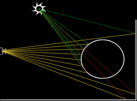 Fig. 1: Point light source In this picture, intersection points of the primary rays with the primitives are used to spawn secondary rays towards the light source to check whether the point is shadowed or not. Red lines are shadow rays that hit something before reaching the light source. Now consider the same scene, but this time with an area light source instead of the point light source: 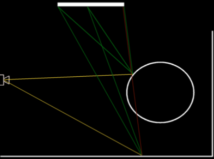 Fig. 2: Area light source I have only drawn two primary rays in this case. The intersection point on the sphere is used to spawn three shadow rays towards the area light. In this case, none of them is occluded, so the point is fully lit by the area light. The intersection point on the floor plane also spawns three rays. This time however only two reach the area light without problems. |
|
Approximating Illumination
|
|
Why three rays? Well, I used three rays because I didn't feel like drawing a hundred green lines, obviously. :) But seriously, to determine how much light an area light casts on a particular spot, you would have to calculate how much of the area of the light source is visible from that point. While this is theoretically possible, it's not exactly practical. Therefore, we approximate the result by sending multiple rays towards the light source and averaging the results. When the number of rays goes to infinity, the solution converges to the correct result. Obviously, an unlimited amount of rays is not practical either, so we will have to find out just how many rays are needed. |
|
Coding Time
|
I moved the code that determines the visibility of a light source as seen from an intersection point to a separate method, 'CalcShade'. Here it is:
Nothing special here, it's the same code as used before. Now let's add some support for area lights:
In this code, 'SPHERE' primitives are still handled as point light sources. Boxes are treated different: A series of rays is cast towards the surface of the box to calculate the average visibility. In the above case, 3x3 rays are generated, so each ray accounts for 1/9th of the full light intensity. Here is a screenshot of the result: 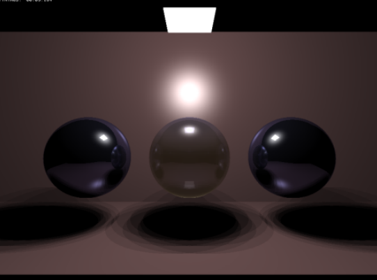 Hmm. Banding. Perhaps we didn't use enough rays? Let's see how 8x8 rays look: 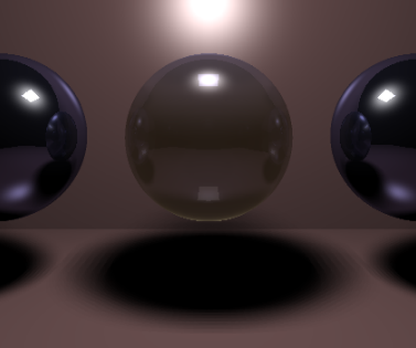 Definitely much better. But, it took 1 minute and 10 seconds to render 3 balls this way. And I still have the feeling that I see some banding, and that this banding would be worse if I zoomed in on the shadow. |
|
Poker Faces and Pimples
|
The banding that you see when sampling 3x3 or 8x8 is caused by the fact that basically you're rendering 9 or 64 shadows. No matter how many samples you take this way, there will always be banding. But there is a better way.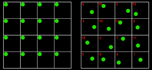 Fig. 3: Random samples In figure three, the left image shows the approach we've taken so far: We took samples in a regular grid. This causes banding. The image to the right shows a different approach: We still use the grid, but inside the grid cells, we use a random offset. This replaces the banding with noise. So is noise better than banding? The answer is: It definitely is. Our eyes are used to noise: When you try to find your way around the house in the dark, you will see plenty of noise as your eyes try to process the faint lighting. I think here some terminology is in place: The above sampling process (using multiple rays to determine a color) is called distribution ray tracing, or Monte Carlo ray tracing. What we are trying to do is to resolve an integral: We are estimating the area of the surface of the light source that we can see from a certain point. This is very hard to solve analytically. Monte Carlo says that when you take enough random samples, the average will converge to the correct solution. In the right image I have numbered the 16 cells. This is useful when you need more than 16 samples: For sample 'x' you can use cell 'x % 16'. This way, you can increase the number of samples without reformatting the grid. Of course, we could also have used a 2x2, or 8x8 or 1x1 grid, but 4x4 seems to be the best balance: 1x1 does not guarantee a good distribution of the rays over the entire area, and neither does 2x2. 8x8 means that we must sample at least 64 rays to cover all cells, and that might be a bit too much in most cases. Here is the modified sampling code:
Some notes about this code: 'SAMPLES' is a constant defined in common.h. When we set it to 32 and 64 the results looks like this: 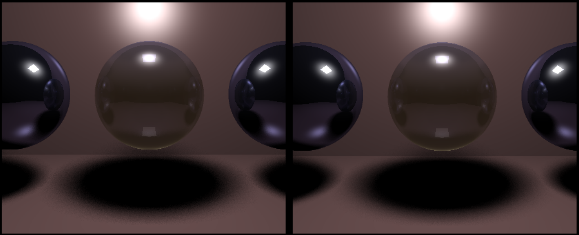 Rendering with 32 samples took 30 seconds; with 64 samples it took 58 seconds. |
|
Diffuse Reflections
|
The same technique can be applied to reflections. Figure 4 illustrates what we are trying to do.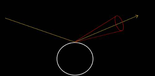 Figure 4: Diffuse reflection Instead of reflecting in a precisely calculated direction, we want to calculate the average of all rays inside the red cone. It would probably look better if there where more rays in the centre of the cone than at the edges, but let's ignore that for a moment. Here is the code that performs the diffuse reflection:
In this code, the original reflection vector (here 'RP') is modified using two perpendicular vectors (RN1 & RN2), scaled by a random value that is not larger than the value set for the diffuse reflection. The 'do...while' makes sure the generated offset is inside the cone. Finally, a lot of rays are cast to determine an estimate of the diffuse reflection. Note that I only perform diffuse reflection for primary rays; otherwise it's just too slow. Also note that the cone is not nicely subdivided like we did for the shadows. The sad result is that the color of the diffuse reflection converges even slower; 128 samples is just barely enough. Here's an image generated using 128 samples: 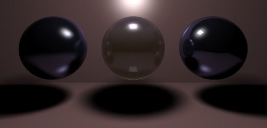 The left sphere is rendered using a diffuse reflection value of 0.6; the middle uses 0.4 and the right one shows perfect reflection. This image took 11 minutes to render... Don't try this at home, kids. :) But it's quite beautiful. |
|
Final Words
|
|
This concludes the fifth installment of the ray tracing column. I tried to make clear that distribution ray tracing is a valuable extension to the basic ray tracing algorithm; it allows for all sorts of cool effects that just can't be done using single rays / secondary rays. Obviously, these techniques require huge amounts of processing power... Or time. As usual, an updated VC6 project is available at the end of this article. You may want to disable the diffuse reflection for the spheres to reduce the rendering time to something reasonable. :) In the next article I will show you how to add texturing and a camera to the raytracer. That's all, have fun! Jacco Bikker, a.k.a. "The Phantom" Links:
|