|
Raytracing Topics & Techniques - Part 6: Textures, Cameras and Speed by (10 November 2004) |
Return to The Archives |
Introduction
 |
|
Welcome to the sixth installment of my ray tracing column. This time I would like to fix some things that I left out earlier: Texturing and a camera. Before I proceed I would first like to correct an error in the previous article. Some readers (Bramz, Thomas de Bodt) pointed out that the way I calculate the diffuse reflection is not correct. Bramz explained that to calculate two perpendicular vectors to the reflected vector, you could use the following method: 1.Pick a random vector V. 2.Now the first perpendicular vector to the reflected vector R is RN1 = R cross V. 3.The second perpendicular vector is RN2 = RN1 cross R. There are some obvious cases where this will not work, but these are easy to work around (e.g., if V = (0,0,1) and R = (0,0,1) then you should pick (1,0,0) for V instead). Also, related to this: The correct term is 'glossy reflection', rather than diffuse reflection. Now that the bugs are out of the way, let's proceed. Perhaps it's good to explain the way these articles are written: Three months back I started working on a raytracer, after reading lots of stuff during my summer holidays. The stuff that interested me most is global illumination, so I pushed forward to get there as fast as possible. This means that I didn't really take a 'breadth-first' approach to ray tracing, but instead built more advanced features upon a simple basis. The raytracer that you see evolving with these articles used to be a very stripped-down version of my own version, with bits and pieces of the full thing being added every week. Last week I added the first feature to the 'article tracer' that was not in the original project (the diffuse reflections). And now I feel it's necessary to add texturing and a free camera, which I also didn't implement yet. The consequence of this is that the code that is included (as usual) with this article is pretty fresh, as it was written specifically for this article. It works though. :) |
|
The Camera
|
|
So far we have worked with a fixed viewpoint (at 0,0,-5) and a fixed view direction (along the z-axis). It would be rather nice if we could look at objects from a different perspective. In modeling packages like 3DS Max this is usually done using a virtual camera. In a ray tracer, a camera basically determines the origin of the primary rays, and their direction. This means that adding a camera is rather easy: It's simply a matter of changing the ray spawning code. We can still fire rays from the camera position through a virtual screen plane, we just have to make sure the camera position and screen plane are in the right position and orientation. Rotating the screen plane in position can be done using a 4x4 matrix. |
|
Look At Me
|
|
A convenient way to control the direction of the camera is by using a 'look-at' camera, which takes a camera position and a target position. Setting up a matrix for a look-at camera is easy when you consider that a matrix is basically a rotated unit cube formed by three vectors (the 3x3 part) at a particular position (the 1x3 part). We already have one of the three vectors: The z-axis of the matrix is simply the view direction. The x-axis of the matrix is a bit tricky: if the camera is not tilted, then the x-axis of the matrix is perpendicular to the z-axis and the vector (0, 1, 0). Once we have two axii of the matrix, the last one is simple: It's perpendicular to the other two, so we simply calculate the cross product of the x-axis and the z-axis to obtain the y-axis. In the sample raytracer, this has been implemented in the InitRender method of the Raytracer class. This method now takes a camera position and a target position, and then calculates the vectors for the matrix:
For once, this is more intuitive in code than in text. :) Note that the y-axis is calculated using the reversed z-axis, the image turned out to be upside down without this adjustment. I love trial-and-error. :) Also note that the rotation part of the matrix needs to be inverted to have the desired effect. |
|
Interpolate
|
|
The matrix is used to transform the four corners of the virtual screen plane. Once that is done, we can simply interpolate over the screen plane. Here is a screenshot of the new camera system in action. Also note the cool diffuse reflection for the floor. 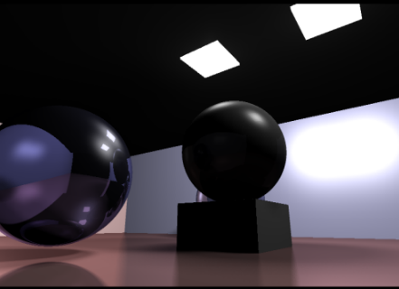 |
|
Texturing
|
|
Looking at the screenshot at the end of the previous paragraph, I really wonder why anyone would want texturing anyway. Graphics without textures have that distinct 'computerish' look to them, a lack of realism that just makes it nicer, in a way. I once played an FPS (I believe it was on an Amiga, might even have been Robocop) that didn't use any texturing at all; all detail like stripes on walls was added using some extra polygons. Anyway. I suppose one should at least have the option to use textures. :) |
|
Texture Class
|
|
I have added some extra code to accommodate this. First, a texture class: This class loads images from disk, knows about things like image resolution and performs filtering. To load a file, I decided to use the TGA file format, as it's extremely easy to load. A TGA file starts with an 18 byte header, from which the image size is easily extracted. Right after that, the raw image data follows. The texture class stores the image data using three floats per color (for red, green and blue). This may seem a bit extreme, but it saves expensive int-to-float conversions during rendering and filtering, and it allows us to store HDR images. |
|
Intersections & UV
|
Next, we need to know what texel to use at an intersection point. In a polygon rasterizer, you would simply interpolate texture coordinates (U, V) from vertex to vertex; for an infinite plane we have to think of something else. Have a look at the new constructor for the PlanePrim primitive:
For each plane, to vectors are calculated that determine how the texture is applied to the plane: one for the u-axis and one for the v-axis. Once we have these vectors, we can fill in the intersection point to obtain the u and v coordinates:
Scaling the texture is now a matter of stretching the u-axis and v-axis for the plane. This is done by multiplying the dot product by a scaling factor, which is retrieved from the Material class. This procedure works well, and we can now apply textures to the walls, ceiling and floor. Note however that this is actually a rather limited way of texturing: We can't set the origin of the texture, and we can't specify an orientation for the texture. Adding this is straightforward though. |
|
Filtering
|
Once the u and v coordinates for an intersection point are calculated, we can fetch the pixel from the texture map and use its color instead of the primitive color. The result looks like this: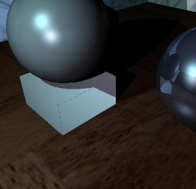 Ouch. That looks like an old software rasterizer. We can easily solve this by applying a filter. There are many filtering techniques, but let's have a look at a simple one: the bilinear filter. This filter works by averaging 4 texels, based on their contribution to a virtual texel. The idea is illustrated in figure 1. 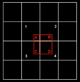 Figure 1: Bilinear filtering The pixel that we would like to fetch from the texture is shown as a red square in the above image. Since we can only get textures at integer coordinates, we get one pixel instead; probably the one labeled as '1' in figure 1. Bilinear filtering considers all four texels covered by the red square. The color value of each texel is multiplied by the area that it contributes to the full texel, so '1' contributes far less then '4'. This is implemented in the following code:
This improves the rendered image quite a bit: 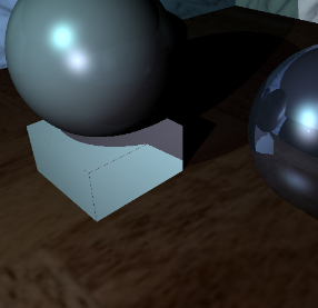 This time the texturing is blurry... Obviously, bilinear filtering is not going to fix problems caused by low-resolution textures, it merely makes it less obvious. Bilinear filtering works best for textures that are the right resolution, and also improves the quality of textures that are too detailed: Using no filter at all would result in texture noise, especially when animating. |
|
Spheres
|
Finally,
let's look at spheres. To determine u and v coordinates at an
intersection point on a sphere, we use polar coordinates, r (the
radial coordinate, or latitude) and T (the angular
coordinate, or polar angle, or longitude).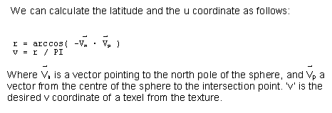 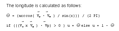 Once we have the u and v coordinates for a texel on the sphere, we can use the same filtering as we used for texturing a plane. The full code:
And an image of the new feature in action:  I'm sure it will look better with a nice earth texture on it. :) |
|
Importance Sampling
|
|
One last thing that I would like to discuss briefly in this article is importance sampling. A recursive raytracer spawns secondary rays at each intersection point. In case of soft shadows and diffuse reflections, this can result in enormous amounts of rays. An example: A primary ray hits a diffuse reflective surface, spawns 128 new rays, and each of these rays probe an area light using 128 shadow rays. Or worse: Each of these rays could hit another diffuse reflective surface, and then probe area light sources. Each primary ray would spawn an enormous tree of rays, and each secondary ray would contribute to the final color of a pixel only marginally. This situation can be improved using importance sampling. For the first intersection, it's still a good idea to spawn lots of secondary rays to guarantee noise-free soft shadows and high quality diffuse reflections. The secondary rays however could do with far less samples: A soft shadow reflected by a diffuse surface will probably look the same when we take only a couple of samples. Take a look at the new method definitions for Engine::Raytrace and Engine::CalcShade (from raytrace.h):
The two new parameters (a_Samples and a_SScale) control the number of secondary rays spawned for shading calculations and diffuse reflections. For diffuse reflections, the number of samples is divided by 4:
'a_SScale' is multiplied by 4 in this recursive call to Engine::Raytrace, sine the contribution of individual rays increases by a factor 4 if we take 4 times less samples. In the new sample raytracer included with this article, perfect reflections spawn only one half of the number of secondary rays that primary rays cast; refracted rays also lose 50% of their samples, and diffuse reflections skip 75%. |
|
Improved Importance
|
| This is only a very simple implementation of importance sampling. You could tweak importance of new rays based on material color (reflections on dark surfaces will contribute less to the final image), on reflectance (a surface that is only slightly reflective requires less precision), the length of the path that a refracted ray takes through a substance and so on. |
|
Final Words
|
Ray tracing is quite a broad subject. Things we have covered so far:
For most of these topics I only scratched the surface of what you can do. For example, besides bilinear filtering there is trilinear filtering and anisotropic filtering, to name a few. You could spend a lot of time on a subject like that. The same goes for Phong: This is really a relatively inaccurate model of how light behaves in real life. You could read up on Blinn or Lafortune, for better models. And then there are the topics that I didn't cover at all, all worth a lifetime of exploration and research: The list is long. And that is good, because it's a wonderful world to explore. It becomes clear however that you can't do it all, unless you make it a full-time job, perhaps. You have to perform importance sampling. :) For the next article I have some very good stuff for you: Highly optimized kd-tree code, pushing the performance of the ray tracer to 1 million rays per second on a 2Ghz machine. The scene from article four is rendered in 1 second using this new code. I will also show how to add triangles to the scene. After that, I have a problem: The writing has caught up with the coding. This means that I am not sure if I will be able to keep the pace of one article each week after article 7. I'll keep you informed. Download: raytracer6.zip See you next time, Jacco Bikker, a.k.a. "The Phantom" |