flipcode - Raytracing Topics & Techniques

Raytracing Topics & Techniques - Part 7: Kd-Trees and More Speed
by (23 November 2004)

Introduction

OK, this is it: The 7th installment of the ray tracing tutorial series. Over the last few weeks I worked very hard to improve the speed of the ray tracer, and I am quite proud of the results: Render times for the scene in article 4 (you know, the sphere grids) dropped from 7 seconds to less than 2 seconds. To put this power to good use, I added a triangle primitive, and a 3ds file loader.

The downside is that the number of changes to the raytracer is enormous. I removed the plane and box primitives, put the triangle and sphere in a single class, removed the regular grid, replaced it with a kd-tree, added a memory manager to align objects in a cache friendly manner, exchanged Phong's expensive pow() for Schlicks slick model, gave the lights their own class and so on. For this article I suggest you unpack the sample code first, you're going to need it while reading this article. As I understand from the feedback that I got that many people like to have the stuff explained without code as much as possible, I'm going to do my best to limit 'code-only' explanations as much as possible.

The good part is that I'm not going to get away with 9 pages in Word for this article (typical size for the previous articles).

Triangles

Before we dive into the hardcore kd-tree generation and traversal, let's first have a look at ray-triangle intersections.

An efficient way to calculate the intersection point of a ray and a triangle is to use barycentric coordinates. It works like this:

First, we calculate the signed distance of the ray to the plane of the triangle. This is the same test that we used for the ray-plane intersections. If the ray does not intersect the plane, we are done (this happens if the ray is parallel to the plane, or starts behind the plane). If the ray intersects the plane, we can easily calculate where this happens, and the problem is reduced to determining whether the intersection point is inside the triangle.

Barycentric Coordinates

This is where the barycentric coordinates come in handy. Barycentric coordinates were invented by mister Möbius (the guy that invented the famous one-sided belt). I'm not covering them in too much detail here; if you want to know all about them then I suggest you check out the MathWorld explanation: http://mathworld.wolfram.com/BarycentricCoordinates.html.

It works like this: Suppose you have a 2D line, from P1 to P2. One way of representing this line is this:

P = P1 + a (P2 – P1)

As long as a is between 0 and 1, we are on the line segment between P1 and P2. We can rewrite the formula like this:

P = a1 P1 + a2 P2

In this formula, a1 and a2 are the barycentric coordinates of point P with respect to the end points P1 and P2. Note that the sum of a1 and a2 must be 1 if we want P to lie between P1 and P2. We can extend this to triangles:

P = a1P1 + a2P2 + a3P3

In this formula, P1, P2 and P3 are the coordinates of the vertices of the triangle, and a1, a2, a3 are the barycentric coordinates of a point in the triangle. Again, the sum of a1, a2 and a3 must be 1. You could visualize it like this: a1, a2 and a3 balance P between the vertices of the triangle.

What makes barycentric coordinates so interesting for ray/triangle intersections is the fact that the barycentric coordinates must all be greater or equal than zero, and summed they may not exceed 1. In all other cases, it's clear that P is not inside the triangle. So, if we know the barycentric coordinates of the hit point, we can accept or reject the ray with very simple tests: Point P is outside the triangle if one of the barycentric coordinates a is smaller than zero, or the summed coordinates are greater than 1.

Calculating the barycentric coordinates can be done like this: First, we start with the previous equation:

P = a1P1 + a2P2 + a3P3

Since the sum of the coordinates must be one, we can substitute a1 with 1 – a2 - a3. A bit of rearranging gives us the following equation:

a2 (P2 – P1) + a3(P3 – P1) = P – P1

This can be solved in 3D, but it's cheaper in 2D. Therefore we project the triangle on a 2D plane. Convenient planes for this are the XY, YZ or XZ planes, obviously. To pick the best one of these, we take a look at the normal of the triangle: By using the dominant axis of this vector we get the projection with the greatest projected area, and thus the best precision for the rest of the calculations.

In 2D a2 and a3 can be calculated as follows:

a2 = (bx hy – by hx) / (bx cy – by cx)
a3 = (hx cy – hy cx) / (bx cy – by cx)

where b = (P3 – P1) and c = (P2 – P1), bx and by are the components of the first projected triangle edge and cx and cy are the components of the second projected triangle edge.

Using the above formulas to calculate the barycentric coordinates for the projected intersection point P the intersection code is now rather simple. In pseudo code:

vector b = vertex3 – vertex1
vector c = vertex2 – vertex1
vector Normal = cross( c, b )
distance = -dot( O – vertex1, N ) / dot( D, N )
// distance test
if (distance < epsilon) || (distance > max_distance) return MISS
// determine dominant axis
if (abs( N.x ) > abs( N.y ))
  if (abs( N.x ) > abs( N.z )) axis = X; else axis = Z
else
  if (abs( N.y ) > abs( N.z )) axis = Y; else axis = Z
// determine project plane axii
Uaxis = (axis + 1) % 3
Vaxis = (axis + 2) % 3;
// calculate hitpoint
Pu = Ou + distance * Du
Pv = Ov + distance * Dv
// check intersection
a2 = (bu * Pv – bv * Pu) / (bu * cv – bv * cu)
if (a2 < 0) return MISS
a3 = (cv * Pu – cu * Pv) / (bu * cv – bv * cu)
if (a3 < 0) return MISS
if (a2 + a3 > 1) return MISS
// ray intersects triangle
return HIT

This approach was suggested by Ingo Wald, in his PhD paper on real-time ray tracing (link at the end of this tutorial). While this method is already pretty fast, it can be done much better. Wald suggests precalculating some data to improve the speed of the algorithm. We can precalculate the dominant axis for each triangle, plus the vectors for the projected triangle edges. Laid out in a way that is perfect for the intersection code:

nu = Nu / Naxis
nv = Nv / Naxis
nd = dot( N, vertex1 ) / Naxis
// first line equation
bnu = bu / (bu * cv – bv * cu)
bnv = -bv / (bu * cv – bv * cu)
// second line equation
cnu = cv / (bu * cv – bv * cu)
cnv = -cu / (bu * cv – bv * cu)

Now the actual intersection code can be simplified like this:

// determine U and V axii
Uaxis = (axis + 1) % 3
Vaxis = (axis + 2) % 3
// calculate distance to triangle plane
d = 1.0f / (Daxis + nu * DUaxis + nv * DVaxis
distance = (nd - Oaxis - nu * OUaxis - nv * OVaxis) * d
if (!(0 < t < maxdistance)) return MISS
// calculate hit point
Pu = OUaxis + t * DUaxis - AUaxis
Pv = OVAxis + t * DVAxis - AUAxis
a2 = Pv * bnu + Pu * bnv
if (a2 < 0) return MISS
a3 = Pu * cnu + Pv * cnv
if (a3 < 0) return MISS
if ((a2 + a3) > 1) return MISS
return HIT

For a detailed derivation I would like to point you to Wald's thesis. The actual implementation of this code for the sample ray tracer is in scene.cpp (method Primitive::Intersect). My implementation is slightly different than Wald's; the method I used requires fewer precalculated values (so it takes less storage), but it does use vertex A to calculate the intersection point. Which method is better depends on whether you add the precalculated values to the primitive class or not; Wald stores these values in a 'TriAccel' structure that contains all the data needed to test for intersections.

Note that the modulo operations at the beginning of this code are quite expensive; you can use a look-up table instead to speed these up.

Normals and Textures

Obviously we are interested in slightly more than just the fact that the ray intersects the triangle. We probably would like to interpolate vertex normals to make the mesh look smooth, and to texture the object, we need to interpolate U and V over the triangle.

Luckily, this is quite simple. Using the barycentric coordinates we can quickly interpolate values over the triangle. Calculating the normal for a given beta and gamma can thus be done as follows:

vector3 N1 = m_Vertex[0]->GetNormal();
vector3 N2 = m_Vertex[1]->GetNormal();
vector3 N3 = m_Vertex[2]->GetNormal();
vector3 N = N1 + m_U * (N2 - N1) + m_V * (N3 - N1);
NORMALIZE( N );
return N;

This code is from method Primitive::GetNormal. It's a bit sad that the interpolated normal requires normalization; this is a significant extra cost.

Calculating U and V is similar; check out Primitive::GetColor for the actual implementation.

Calculating Vertex Normals

To interpolate vertex normals, you need to have those available, obviously. I used an extremely simple 3ds loader that does not import things like smooth groups and stuff like that (I didn't want to turn this project into a 3ds file loading project), so I needed some code to quickly generate these normals.

A vertex normal is calculated by averaging the directions of the normals of all faces that the vertex belongs to. A naïve implementation can be really slow: For each vertex, you scan all faces to see if the vertex is used in that face, and if so, you add the face normal to a vector that accumulates these normals. Once you have checked all the faces, you normalize the accumulated vector to get the final vertex normal.

A programmer that worked on 3d studio once sent me an e-mail, suggesting a faster method:

While reading the mesh, make a list of faces that each vertex uses. This can be done without slowing down the loading: Each time a vertex is used to create a face, this face is added to a list of faces for that vertex. Once the object is loaded, you have for each vertex a list of faces that use that particular vertex. Calculating the vertex normal is now a matter of summing the normals of these faces and normalizing. This gives you the vertex normals virtually for free. The actual implementation is 'interesting' (as in 'challenging'): It requires an array of pointers to primitives per vertex, so the array declaration looks as follows:

Primitive*** vertface = new Primitive**[m_NrVerts];

If you ever used the even more complex '****' in a real-world application, I would like to hear from you. :)

You can check out the tiny 3ds loader and vertex normal calculation code in scene.cpp.

Here is a screenshot of an earlier scene, combined with a triangle mesh: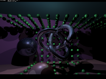

Kd-trees

The triangle intersection code that I explained is fast. Very fast, in fact: The version with the precomputed data is twice as fast as the Möller-Trumbore code that everyone seems to be using. I think my ray-sphere intersection code is still faster, but spheres are not very useful for generic scenes.

So now we are ready for the next step: Implementing a better spatial subdivision scheme, so that we find the right triangle as quickly as possible. Vlastimil Havran did an extensive study of available spatial subdivision schemes (including regular grids, nested grids, octrees and kd-trees) and concludes in his thesis that the kd-tree beats the other schemes in most cases. And Ingo Wald claims that it is possible to limit the number of ray-triangle intersections to three or less using a well-build kd-tree.

Building a Kd-tree

A kd-tree is an axis-aligned BSP tree. Space is partitioned by splitting it in two halves, and the two halves are processed recursively until no half-space contains more than a preset number of primitives. While kd-trees may look like octrees at first, they actually are quite different: An octree always splits space in eight equal blocks, while the kd-tree splits space in two halves at a time. The most important difference though is that the position of the splitting plane is not fixed. In fact, positioning it well is what differentiates a good kd-tree from a bad one. Consider the following images: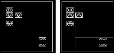

The left image shows a scene with some objects in it. In the right image, this scene is subdivided; the first split is the vertical line, then both sides are split again by the horizontal lines. The split plane position is chosen in such a way that the number of polygons on both sides of the plane is roughly the same.

While this may sound like a good idea at first, it actually isn't: Imagine a ray traversing this scene; it will never pass through an empty voxel. If you keep adding planes to this tree using the same rule, you'll end up with a tree that does not contain a single empty node. This is pretty much the worst possible situation, as the raytracer has to check all primitives in each node it travels through.

Now consider the following subdivision: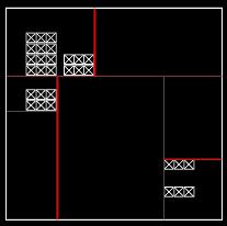

This time, a different rule (or 'heuristic') has been used to determine the position of the split plane. The algorithm tries to isolate geometry from empty space, so that rays can travel freely without having to do expensive intersection tests.

A good heuristic is the SAH – or surface area heuristic. The basic idea is this: The chance that a ray hits a voxel is related to it's surface area. The area of a voxel is:

area = 2 * width * height * depth

The cost of traversing a voxel can be approximated by the following formula:

cost = Ctraversal + area * prims * Cintersect

Since splitting a voxel always produces two new voxels, the cost of a split at a particular position can be calculated by summing the cost of both sides.

The split plane position that is the least expensive is then used to split the voxel in two new voxels, and the process is repeated for these voxels, until a termination criterion is met: The process can for example be halted when there are three or less primitives in the voxel, or when the recursion depth is 20 (these are values that I use right now).

An interesting extra termination criterion follows from the cost function: If the cost of splitting the voxel is higher than leaving the voxel as it is, it is also a good idea to stop splitting.

Implementation

OK, that was a lot of theory. But it's worth the trouble: Moving from a regular grid to a naïve kd-tree implementation almost doubled the speed. Moving from a simple heuristic to the SAH doubled the speed again.

So let's have a look at the actual implementation of the kd-tree construction algorithm. Building a kd-tree generally looks like this, in pseudo-code:

void buildkdtree( Node* node )
{
	if (stopcriterionmet()) return
	splitpos = findoptimalsplitposition()
	leftnode = new Node()
	rightnode = new Node()
	for (all primitives in node)
	{
		if (node->intersectleftnode()) leftnode->addprimitive( primitive )
		if (node->intersectrightnode()) rightnode->addprimitive( primitive )
	}
	buildkdtree( leftnode )
	buildkdtree( rightnode )
}

Building a tree is really that simple. The first version of the kd-tree compiler for the sample raytracer was a mere 40 lines of code. There are some tricky parts though: Finding the split plane position using SAH, and checking intersection of a primitive and an axis aligned box.

Box-primitive Intersections

If you go back to one of the previous versions of the sample ray tracer, you can see that box-sphere intersections are handled by checking the box against the bounding box of the sphere. This is not optimal. Consider the following situation: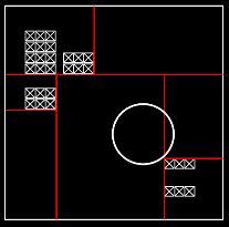

Does this box intersect the lower-right voxel? Using the old test it does. And that's not good; every ray that visits the lower-right voxel will check intersection with the sphere. I found a better method on a site with BlitzBasic code snippets:

bool Primitive::IntersectSphereBox( vector3& a_Centre, aabb& a_Box )
{
	float dmin = 0;
	vector3 spos = a_Centre;
	vector3 bpos = a_Box.GetPos();
	vector3 bsize = a_Box.GetSize();
	for ( int i = 0; i < 3; i++ )
	{
		if (spos.cell[i] < bpos.cell[i]) 
		{
			dmin = dmin + (spos.cell[i] - bpos.cell[i]) * (spos.cell[i] - bpos.cell[i]);
		}
		else if (spos.cell[i] > (bpos.cell[i] + bsize.cell[i])) 
		{
			dmin = dmin + (spos.cell[i] - (bpos.cell[i] + bsize.cell[i])) * (spos.cell[i] - (bpos.cell[i] + bsize.cell[i]));
		}
	}
	return (dmin <= m_SqRadius);
}

I'm not terribly in the exact details of this code, so if you don't mind I'm just going to accept that it works.

Initially I used a similar simplification for triangles. You can check the new box-triangle intersection in scene.cpp, I used the version made by Tomas Akenine-Möller (the same guy that worked with Trumbore on ray/triangle intersections), as it's fast and short. The effect on the performance of the ray tracer is dramatic. Without the improved box/primitive intersection code, each ray was checked against 22 primitives on average. With the new code, this figure went down to 6.7. VTune made the impact even clearer: Without proper box/primitive intersection code, the intersection tests took 80% of the clock cycles (compared to 15% for the traversal code). With the new code, the same amount of time is spent inside the intersection code as in the traversal code.

The impact on rendering speed is dramatic, as expected: The scene from article 4 now renders in less than a second when rendering to a 512x384 canvas.

Implementing SAH

Let's go back to the formula for the cost of a single voxel using the surface area heuristic:

cost = Ctraversal + area * prims * Cintersect

This is the cost for a single voxel. The cost of a voxel after splitting it is the sum of the cost of the two new voxels:

cost = costleft + costright

To find the optimal split position, we have to check them all. Luckily, the number of interesting split plane positions is limited: A split plane should always be situated at the boundary of a primitive. All other positions don't make sense, since the number of primitives won't change between two primitive boundaries. Sadly, even with this restriction, the number of candidate split plane positions is daunting. Imagine a scene containing 8000 triangles. For the first split, we have to consider roughly 16000 positions. For every position, we need to count the number of primitives that would be stored in the left and right voxel.

In pseudo code:


bestpos = -1
bestcost = 1000000
for (each primitive in node)
{
	left_extreme = primitive->getleftextreme( axis )
	right_extreme = primitive->getrightextreme( axis )
	if (cost = calculatecost( left_extreme ) < bestcost)
	bestcost = cost, bestpos = left_extreme
if (cost = calculatecost( right_extreme ) < bestcost)
	bestcost = cost, bestpos = right_extreme
}

float calculatecost( splitpos )
{
	leftarea = calculateleftarea( splitpos )
	rightarea = calculaterightarea( splitpos )
	leftcount = calculateleftprimitivecount( splitpos )
	rightcount = calculaterightprimitivecount( splitpos )
	return costtrav + costintersect * (leftarea * leftcount + rightarea * rightcount)
}

You can check out the actual implementation in the sample ray tracer project. I tried some things to speed up the code: The candidate split plane positions are first stored in a linked list. During this first loop, duplicate positions are eliminated, and the positions are sorted.

In a second loop, the left and right voxel primitive counts are calculated for each split plane position. This is where the sorted list comes in handy; as we are walking from left to right, we can tag primitives that are to the left of the current plane, so we can skip them in the next iteration.

Even using these tricks the kd-tree compiler is too slow. If someone has a good suggestion to improve this, I would like to hear it. :)

The generated tree is quite good however. It can be improved, consider this work in progress: Right now, triangles are not clipped to the parent voxel before their extends are determined. Doing this clipping allows split planes to be situated at the exact position where a triangle leaves a node. This is not a very difficult extension, but it will make the tree compiler even slower.

Traversing the Kd-tree

To traverse the kd-tree, I implemented Havran's TA^B_rec algorithm (Havran tried a lot of spatial subdivisions and traversal algorithms; TA stands for 'traversal algorithm', rec means recursive and B is the version – His code is a modification of an existing algorithm A). The code is not overly complex, but instead of copying a huge amount of text from his thesis I rather point you to the original document.

Ingo Wald apparently found an even more efficient way to traverse a kd-tree, but in my experience, his implementation suffers badly from numerical stability problems. His implementation notes are quite sketchy (which is why I didn't feel so guilty about heavily quoting his work) and he only mentions these problems, without the solutions. Wald on the other hand designed his approach specifically to cope with stability issues.

The actual code is much smaller than the regular grid traversal code, which is a nice bonus. :)

Finetuning

Once the ray tracer is in good shape algorithm-wise, it's time to revert to old-skool hardcore optimizing.

Check out the class declaration of the KdTreeNode (I know, it's code, but it's interesting):


class KdTreeNode
{
public:
	KdTreeNode() : m_Data( 6 ) {};
	void SetAxis( int a_Axis ) { m_Data = (m_Data & 0xfffffffc) + a_Axis; }
	int GetAxis() { return m_Data & 3; }
	void SetSplitPos( real a_Pos ) { m_Split = a_Pos; }
	real GetSplitPos() { return m_Split; }
	void SetLeft( KdTreeNode* a_Left ) { m_Data = (unsigned long)a_Left + (m_Data & 7); }
	KdTreeNode* GetLeft() { return (KdTreeNode*)(m_Data&0xfffffff8); }
	KdTreeNode* GetRight() { return ((KdTreeNode*)(m_Data&0xfffffff8)) + 1; }
	void Add( Primitive* a_Prim );
	bool IsLeaf() { return ((m_Data & 4) > 0); }
	void SetLeaf( bool a_Leaf ) { m_Data = (a_Leaf)?(m_Data|4):(m_Data&0xfffffffb); }
	ObjectList* GetList() { return (ObjectList*)(m_Data&0xfffffff8); }
	void SetList( ObjectList* a_List ) { m_Data = (unsigned long)a_List + (m_Data & 7); }
private:
	// int m_Flags;
	real m_Split;
	unsigned long m_Data;
};

I bet this looks extremely obscure. :) There is a reason for this though: To optimize cache behavior, I tried to reduce the amount of space that a single KdTreeNode uses to 8 bytes. That means that 4 KdTreeNodes fit in a single cache line. The data for a KdTreeNode is laid out in a peculiar manner: First, there is the split plane position, a float that uses 4 bytes. The other data member is 'unsigned long m_Data'. This field actually contains three values: A pointer to the left branch, a bit indicating whether this node is a leaf or not, and two bits that determine the axis for the split plane. A pointer to the list of primitives in a leaf node is also available: Since a leaf node does not need a pointer to it's left and right kids, this space can be used for a pointer to the primitive list.

Since the object takes 8 bytes, it's good for the cache to align the address for each node to an 8 byte boundary. That also means that the lower three bits of every KdTreeNode pointer are zeroes. These bits can thus be used for other purposes, but only if addresses are properly masked when they are needed. That is the reason for the bitmasks in many of the methods: These bitmasks simply filter out the requested data.

The multiple-of-8 addresses for KdTreeNodes are enforced by a custom memory manager. This manager allocates a large chunk of memory, and returns new KdTreeNodes upon request.

I already mentioned that the m_Data field also contains one implicit value: A pointer to the right branch. KdTreeNode allocations are always done in pairs: This guarantees that the address of the right branch KdTreeNode is always 4 bytes more than the left branch KdTreeNode. Now all required data fits in 2 dwords.

Further Improving Cache Performance

One other small thing that I added to improve cache behavior is tiled rendering: Instead of drawing entire scanlines at a time, the new sample ray tracer renders tiles of 32x32 pixels. You may think that this can't possibly have a big impact on the performance of the ray tracer, but the opposite is true: The impact on rendering time is no less than 10%.

This can be explained: When sending rays in bundles, they are much more likely to use the same data. Many rays that share a tile will also hit the same voxels and possibly also the same primitives. I have to admit that the impact on performance did surprise me.

I tried various configurations, but 32x32 tiles seem to give the best performance.

Future Work

So much to do, so little time. And I just bought Half Life 2, so that's not going to help either. :)

Future work can be divided in two main branches:

First, the ray tracer can be made much faster. Don't get me wrong, the current ray tracer is quite fast, and does not use any tricks that limit it's usability. It's a solid basis for future development. However, Wald is reporting speeds of several frames per second for scenes consisting of thousands of polygons at a resolution of 1024x768 pixels, on a single 2.5Ghz laptop. That would mean that I am at only 20% of his speed. A coders nightmare... The biggest gain could be obtained by tracing ray packets of 4 rays simultaneously; this makes the algorithm exceptionally suitable for SSE optimizations. Even without SSE code this approach is interesting: Since all rays in the packet use the same data, the amount of data that is used by the ray tracer is reduced considerably. Wald reports speedups of 200-300% using this approach.

Second, there's functionality. The current ray tracer really is a bare bones program. I would really like to work on global illumination (like I promised), and on materials (bump maps, BRDF's), or on real-time ray tracing.

Right now the plan is to let the performance issue rest for a while. After I complete Half Life 2 I would like to integrate the photon mapping code that I did earlier in the current ray tracer. That's going to take some time, as my knowledge of ray tracing evolved considerably. It was quite a ride. :)

Last Words

That's it for the moment. At the end of this article you will find a download link to raytracer7.zip, Wald's thesis and Havran's thesis. Both documents are very good reads, so if you didn't check them earlier, do so now.

Thanks for your attention, and see you soon.

Jacco Bikker, a.k.a. "The Phantom"

Links:
"Heuristic Ray Shooting Algorithms", Vlastimil Havran:
http://www.cgg.cvut.cz/~havran/phdthesis.html

"Real Time Ray Tracing and Interactive Global Illumination", Ingo Wald:
http://www.mpi-sb.mpg.de/~wald/PhD/

And the latest VC6 project: raytracer7.zip

Article Series:

Raytracing Topics & Techniques - Part 1 - Introduction
Raytracing Topics & Techniques - Part 2 - Phong, Mirrors and Shadows
Raytracing Topics & Techniques - Part 3: Refractions and Beer's Law
Raytracing Topics & Techniques - Part 4: Spatial Subdivisions
Raytracing Topics & Techniques - Part 5: Soft Shadows
Raytracing Topics & Techniques - Part 6: Textures, Cameras and Speed
Raytracing Topics & Techniques - Part 7: Kd-Trees and More Speed