|
Raytracing Topics & Techniques - Part 2 - Phong, Mirrors and Shadows by (06 October 2004) |
Return to The Archives |
Introduction
 |
|
In the first article I described the basics of raytracing: Shooting rays from a camera through a screen plane into the scene, finding the closest intersection point, and simple diffuse shading using a dot product between the local normal of the primitive and a vector to the light source. In the second article I would like to introduce you to mr. Phong, his bathroom mirrors and his shady sides. :) For years I actually believed that 'phong' had something to do with the 'pong' sound that photons make when they bounce off a surface (if you listen really carefully), and I also believed that phong is normally implemented using a texture with a bright spot on it. But that appears to be phake phong... |
|
Primary vs Secondary Rays
|
Consider the following image: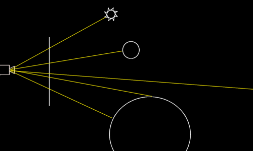 Fig. 1: Primary rays This image shows the rays that the simple raytracer from the first article shoots into the scene. A ray can hit a light source, or a primitive, or nothing. There are no bounces and no refractions. These rays are called 'primary rays'. Besides primary rays, you can use 'secondary rays'. These are shown in the next image (don't faint): 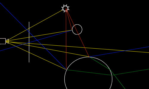 Fig. 2: Various types of secondary rays The blue lines in this picture are reflected rays. For reflection, they simply bounce off the surface. How to do that exactly will be addressed in a moment. The green lines are refracted rays. These are a bit harder to calculate than reflected rays, but it's quite doable. It involves refraction indices and a law formulated by mr. Snell (also known as Snellius, which is a rather strange habit of people of his period of time; imagine I called myself Phantomius ñ That would be odd). The red lines are rays used to probe a light source. Basically, when you want to calculate the diffuse lighting, you multiply the dot product by 1 if the light source is visible from the intersection point, or 0 if it is occluded. Or 0.5 if half of the light source is visible. If you follow one of the yellow rays starting at the camera, you will notice that each ray spawns a whole set of secondary rays: One reflected ray, one refracted ray and one shadow ray per light source. After being spawned, each of these rays (except for shadow rays) is treated as a normal ray. That means that a reflected ray may be reflected and refracted again, and again, and againÖ This technique is called 'recursive raytracing'. Each new ray adds to the color that its ancestor gathers, and so finally each ray contributes to the color of the pixel that the primary ray was originally shot through. To prevent endless loops and excessive rendering time, there is usually a limit on the depth of the recursion. |
|
Reflections
|
To reflect a ray of a surface with a known surface normal, the following formula is used:
(where R is the reflected vector, V is the incoming vector and N is the surface normal) This is implemented in the following code, which can be added to the raytracer right after the loop that calculates the diffuse illumination per light source.
If you didn't change the scene of the sample raytracer, you should now have something like this: 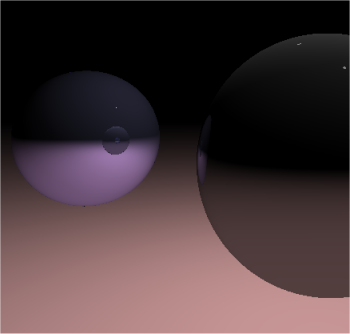 And that's quite an improvement. Note that both spheres reflect each other, and that the spheres also reflect the ground plane. |
|
Phong
|
|
Creating 'perfect' lighting is extremely complex, so we will have to revert to an approximation. While the diffuse shading we used so far is excellent for soft looking objects, it's not so great for shiny materials. Besides, it doesn't give us any control at all, other than the intensity of the lighting. Take a look at the following images: 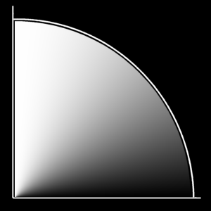 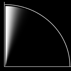 Fig. 3: Diffuse versus specular lighting The left image shows the lighting that we used so far: The dot product of the normal and the light vector. There is a linear transition from white to black. On the right side you see a graph of the same dot product, but this time raised to the power 50. This time, there is a very bright spot when the two vectors are close, and then a rapid falloff to zero. Combining these improves matters quite a bit already: We get quite a bit of flexibility. A material can have some diffuse shading, and some specular shading; and we can set the size of the highlight by tweaking the power. It's not quite right though. The diffuse shading is OK: A diffuse material scatters light in all directions, and so its brightest spit is exactly there where the material faces the light source. Taking the dot product between the normal and a vector to the light gives this result. Specular shading is a bit different: Basically, the specular highlight is a diffuse reflection of the light source. You can check this in real life: Grab a shiny object, put it on a table under a lamp, and move your head. You will notice that the shiny spot does not stay in the same position when you move: Since it's basically a reflection, its position changes when the viewpoint changes. Phong suggested the following lighting model, that indeed takes the reflected vector into account:
(where L is the vector from the intersection point to the light source, N is the plane normal, V is the view direction and R is L reflected in the surface) Notice that this formula covers both diffuse and specular lighting. The code that implements this is shown below.
After adding this to the lighting calculation, the raytracer produces an image like the one below: 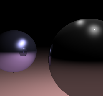 Which is quite an improvement. |
|
Shadows
|
|
The last type of secondary ray is the shadow ray. These are a bit different than the others: they do not contribute directly to the color of the ray that spawned them; instead they are used to determine whether or not a light source can 'see' an intersection point. The result of this test is used in the diffuse and specular lighting calculations. The code below creates a shadow ray for each light source in the scene, and intersects this ray with all other objects in the scene.
Most of this should be familiar by now. The result of the test is stored in a floating point variable 'shade': 1 for a visible lightsource, and 0 for an occluded light. Using a float for this might seem odd; however later on we will add area light sources, and those are often only partially visible. In that case, a 'shade' value between 0 and 1 would be used. By the way, the above code does not always find the nearest intersection point of the shadow ray with the primitives in the scene. This is not necessary: any intersection with a primitive that is closer than the light source will do. This is quite an important optimization, as we can break the intersection loop as soon as an intersection is found. Picture: 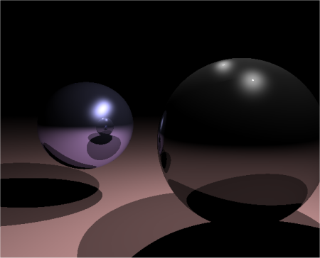 And there you have it. Two raytraced spheres, reflections, diffuse and specular shading, shadows from two light sources. The lighting on the plane subtly falls off in the distance due to the dot product diffuse lighting, resulting in a nice shading on the spheres. And all this renders within a second. Notice how the shadows overlap to make the ground plane completely black. Notice how the color of the spheres affects the reflected floor plane color. Raytracing is addictive, they say. :) |
|
Final Words
|
|
One of the cool things about raytracing is that if you plug in something new, all the other things still work. For example, adding shadows and Phong highlights also adds reflected shadows and highlights. This is probably related to the parallel nature of raytracing: Individual rays are quite independent, which makes recursive raytracing very suitable for rendering on multiple processors, and also for combining various algorithms. By the way, there's an error in the raytracer, which I will fix for the third revision: The result of the shadow test that is used for the diffuse component is also used for the specular component. Obviously, this is wrong. :) Send your solutions for great prizes and eternal fame! That's all for the second article. Next up: Refractions, Beer's law and adaptive supersampling. An updated raytracer project is available using the link at the bottom of the page. Greets, Jacco Bikker, a.k.a. "The Phantom" Link: Sample project 2 ñ raytracer2.zip |