|
Theory & Practice - Issue 03 - Curved Surfaces by (31 May 2000) |
Return to The Archives |
Introduction
 |
|
Recently there has been a lot of hype about curved surfaces, mostly due to games
like Quake III and Messiah, although engines such as Crystal Space had their own
curved surfaces earlier. Overall, curved surfaces provide a good structure to
store information about shapes. As 3D environments get more and more detailed it
becomes more important to organize information in a way that allows simple
description and manipulation. You can, for example, build lots of little
polygons instead of having a curved surface, but that would be much more
information to store, and also not very manageable if you wanted to change the
curve later on. Using curved surfaces is also better for implementing
Level-Of-Detail optimizations, which I will talk about later. In a sense, curved
surfaces are the vector graphics of the 3D world. This time, I'm going to introduce curved surfaces and how to implement them. |
In General
 |
|
There are two main aspects to curved surfaces: how their information is defined
and how they are rendered. There are different methods for defining curved
surfaces, including Bezier patches (pronounced "Bez-yeah") and NURBS
(Non-Uniform Rational B-Spline). I am going to talk about Bezier patches a bit,
but then I'll focus on another method which I use, which is really neither
Bezier nor B-spline surface. Both methods are based on 2D Bezier curves, which
we will discuss first. When times comes to draw, it all boils down to tesselating curved patches into flat triangles. The current 3D cards do not support actual curved surface texturemapping, so you have to approximate the curves with the flat triangles which the cards can texturemap. What tesselation means and how it is done will be discussed below. |
Smooth Sailing
 |
We will first explore 2-dimensional Bezier curves, which is a good place to
start. It's often good to learn a technique in the context of solving a problem,
and this time we'll do just that. Suppose you had a 2D landscape, and you didn't
have enough space to record the height at every single pixel. Instead, in which
you had the height recorded every 20 pixels. When drawing this landscape, you
could get the points every 20 pixels and connect them with lines. You'd end up
with a somewhat blocky approximation of the actual landscape: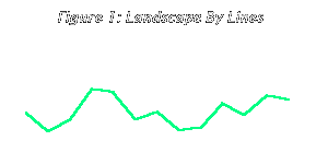 Someone viewing this might notice the rough edges and would consider this undesirable. If we could smooth things out the landscape would look much more natural. What we want is a smooth curve that goes through all the points in the heightmap. 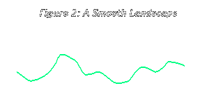 We realize that a smooth landscape has a tangent vector at every point. It therefore also has a normal (perpendicular) vector at every point. If we could record, say, the normal or tangent vector for every known point in the heightmap, we could create a smooth surface by interpolating the slope of the landscape between any two known points. 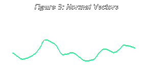 So our landscape will consist of a series of small curves, which we can refer to as 2D patches. If we have two points and two tangents, we can draw a Bezier curve that interpolates linearly between those tangents. 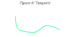 By the way, we can actually calculate a natural normal vector at every point in the heightmap, instead of storing the extra normal vector data along with the vertex data. In this case for any point Pn the normal vector would be the average of the vectors (Pn->Pn-1) and (Pn->Pn+1). However, if we want to have unnatural-looking normal vectors at some points we will have to store them for the 3D engine, since how is the engine supposed to know what we want? In short, given a series of points of a heightmap (and no extra data) you can make a smooth landscape that goes through them, but if you want to control the slant of the landscape your own way at some points then you have to store the normal vectors or tangent vectors. Given the series of 2D points, we can calculate a smooth curve that runs through them using spline curves. Instead, though, I am going to discuss how to accomplish this using Bezier curves, which I think is easier to explain. Both methods result in pretty much the same curve, but they differ in how the curve is defined. |
Bezier Curve Math
 |
|
Now, onto the mathematics of it all. How to draw a curve from two points and two
tangent vectors? Bezier curves can be specified with three or more control
points. The curve begins at the first control point, and ends at the last
control point. The control point(s) in between control its curvature and
direction, basically altering it from what would otherwise be a straight line. We can obtain the four points necessary for drawing a cubic Bezier curve from our two points and two tangent vectors. 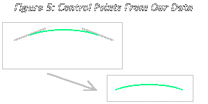 By varying these points, we can vary the curve. Now I will talk about how to actually calculate the curve based on the control points. There are several ways of doing this, and the simplest to explain is probably the deCasteljau algorithm. First, let us consider the control points specified. The Bezier curve starts at the first control point, and ends at the last control point in the sequence. Think of the curve as a path along which a particle travels. At time t=0, the particle is at the first control point, and at time t=1, the particle is at the last control point. The Bezier curve is the path traced out by the particle as it travels from the first to the last control point. So how do we find this path? We use the deCasteljau algorithm. The algorithm, simply put, consists of repeated interpolation. Suppose we want to know where the particle is at a time t, 0 <= t <= 1. We use interpolation to find the contribution of each of the control points to the particle's position. The short answer for those of you who don't want the hows and whys, is the equation: (1) P(t) = (1-t)3 * P0 + 3t(1-t)2 * P1 + 3t2(1-t) * P2 + t3 * P3 Just plug the points into this equation, and the time (say, 0.5), and you get the position of the particle at that time. Here is the math behind the deCastlejau algorithm: 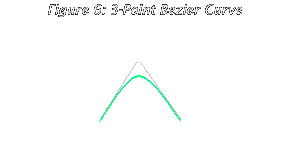 Let's begin with a Bezier curve described by 3 points in the x-y plane: P0 = (0, 0), P1 = (2, 4), and P2 = (4, 0). Now suppose that we want to know where the particle is at time t = 0.5. We start by interpolating between P0 and P1. We will call Pi1 the result of interpolating between points Pi and Pj. Later, we will call Pi2 the result of interpolating between points Pi1 and Pj1, and so forth. Let's look at the mathematics of this process. To interpolate between P0 and P1, we see that P01(t) = P0 + t (P1 - P0). Similarly, we see that P11(t) = P1 + t (P2 - P1). The final step in this process is to interpolate between P01 and P11: P02(t) = P01 + t (P11 - P01). The result of interpolating between P0 and P1 is P01 = (1, 2). Next, we interpolate between P1 and P2 to find P11 = (3, 2). Finally, we interpolate between P01 and P11 to find P02 = (2, 2). Thus, the position of the particle at time t = 0.5 is (2, 2). We can draw the entire curve by repeating this process for values of t ranging from zero to one. 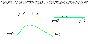 Let's return to the equations above for a minute. Suppose that we substitute the first two equations into the third. This gives us the equation: P02(t) = (1-t)2 * P0 + 2t(1-t) * P1 + t2 * P2 Note that this is a quadratic equation in t. Thus, three Bezier control points may be used to define a quadratic curve. This follows directly from the fact that we used two successive rounds of linear interpolations to find the particle's position. It then follows that for four Bezier points, we would need three rounds of linear interpolation, which would produce a cubic equation. Thus, four Bezier points may be used to define a cubic curve. More generally, n+1 Bezier points may be used to define uniquely a polynomial curve of degree n. This polynomial is given by the equation:
where:
The Berenstein polynomials are given by
A quick note: the "n!/[i!*(n-i)!]" part produces everyone's favorite Pascal triangle. :-) So, for example, for four control points the equation would be equation (1), presented above. Suppose that after each round of interpolation, we drew lines connecting the newly interpolated points that were adjacent to each other. That is, we connected P11 and P21, and then we connected P21 and P31, and so forth. In effect, we would be drawing a new control polygon at each step. This succession of lines will eventually converge to the Bezier curve. 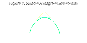 That's the idea behind the deCastlejau algorithm. If you have Java enabled, play around with this applet. It gives you a very good idea of what's going on when you're drawing Bezier curves using the algorithm. Let's concern ourselves with one more problem, and that is: given a particular t, we want to find the slope of the curve at that t. A Bezier curve is smooth (differentiable at every point) so we can get its slope at any point. We do that as follows. Recall the deCastlejau algorithm. Suppose a curve consists of four control points. We want to find out the tangent vector to the curve at some t. We proceed as we would if we wanted to find the position of the curve at that t. We interpolate the four points into three points, and the three points into two points. Now, however, instead of interpolating the two points into one point, we just look at the line that goes through the two points, since that's the tangent line to the curve at that t. So, how do we get these two points that define the line? Suppose you had a Bezier curve defined by n control points, and a t between 0 and 1. You take the curve defined by the first n-1 control points, and find its position at t. Then you take the curve defined by the last n-1 control points and also find its position at t. That gives you the two points that define the line you're looking for. Take a look at the picture to understand this visually: 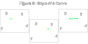 |
What About 3D?
 |
|
Alright, now onto 3D curves surfaces. First I will explain the Bezier patch and how it works. Recall that a cubic Bezier curve is defined by 4 points. A cubic Bezier patch is defined by 16 points. They are arranged like this: 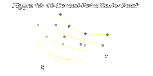 Basically this is interpreted as 4 Bezier curves (the white curves). The control points control both the "horizontal" and the "vertical" Beziers. You have two parameters now -- s and t (instead of just t) -- running in orthogonal directions. Let's say s runs "horizontally" and t runs "vertically". To calculate the position of any point on the Bezier patch, given s and t, you first interpolate the positions of the four Bezier curves oriented horizontally, given s. From this you obtain four points -- the positions of the four "particles" given that s. Using these positions you find the point on the resulting vertical Bezier curve. That's where the point should be on the Bezier surface. Alternatively, you could evaluate the vertical Bezier curves first, obtain the control points for the horizontally oriented Bezier, and evaluate that. No matter whether you do s or t first, you should get the same point. You can also get the slope at any point by calculating the partial derivatives of the polynomial curve. Here's how you actually draw a Bezier surface (and texturemap it if you want). Pick some interval for s and some interval for t. The interval depends on the number of steps you want. For example, if you want 5 steps in s you'd have the interval be 1/5 = 0.2 . Then you generate the vertices for the flat polygons. For each s and for each t you go through the patch and you calculate the position of the next vertex. What you end up with is an M by N set of connected quads. These quads are what you draw and texturemap. Now, I am going to talk about another method of curving surfaces. I often try to solve problems on my own, and I developed this method before I really read much documentation on Bezier patches, NURBS surfaces, etc. So I don't think it's exactly like any other method, but it works very well. The method I use is based on the idea of curved primitives. The edges of a polygon are stored as Bezier curves, and the curvature is interpolated between the edges across the polygon's surface. What you do is break it into curved triangles and tesselate them. Now, every vertex has two tangent vectors. One tangent vector corresponds to one edge that touches the vertex, and the other vertex corresponds to the second edge. Using these, we can obtain Bezier curves along the edges. 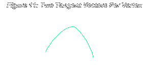 If an edge has both tangent vectors as (0, 0) there is no curvature in that edge, 2nd and 3rd Bezier points are the same as the 1st and 4th. If the four control points for a Bezier edge lie on a plane, then the edge is said to "curve naturally". It's like holding a triangular piece of paper by its corners and bending it. See how the paper curves. Here's how a curved triangle would look compared to a flat triangle: 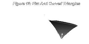 Now we know how to store the data for the curved triangle. How do we draw it? We do it by tesselation into flat polygons, similar to the Bezier patch. This time, though, we can do this linearly or fractally. |
Fractal Tesselation
 |
We can split one triangle into four using the following pattern: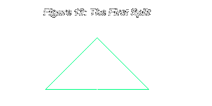 Some of the vertices for the four triangles are the original triangle's vertices. The rest are, actually, the midpoints of the edges of the original triangle. Since for each edge we have the equation for its Bezier curve, we can find the midpoint simply by taking t = 0.5 . Now that we know the positions of the midpoint vertices, we need to generate tangent vectors for them. The tangent vector for each midpoint vertex is the slope of the edge it's created on, at the time 0.5 . We only need to keep one tangent vector for each "child vertex", as opposed to two for the original triangle's vertices. All the edges for which a child vertex is a vertex will use the child vertex's tangent vector -- the only one it has. This is because whoever designs the original triangle might want a great deal of flexibility in defining its shape, but when we create the child vertices there is only one curve per edge, so we need no flexibility there. If you want to texturemap the triangle, each child vertex gets the average of the u and v from its parent vertices. The same gose for most other qualities you want to interpolate across the curved surface. Anyway, when the split is complete we obtain four new curved triangles. You continue to split these fractally into smaller and smaller triangles, until you reach the level of detail you want: 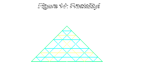 Now, how do you store the newly created vertices in RAM? Since RAM is linear memory, we need to develop a scheme to store the fractal's vertices, in the order they are created. So you first store the 3 original vertices, then the 3 new vertices obtained from the first split, then the 9 new vertices obtained from the second split, etc. How do we know how many new vertices are created after each split? It's not very hard. We notice that each new batch of vertices created after a split can be grouped in groups of 3, forming upside-down triangles (take a look at the picture above -- first the white, then the yellow, then the blue). And from that we see that the number of these upside-down triangles after the nth split will be the nth triangular number. I hope you know what triangular numbers are, but if you don't, the nth triangular number is how many dots would be arranged in a triangle with n dots at the base, n-1 dots above that, etc., and is given by the expression: nth triangular number = n(n+1) / 2 Anyway, we see that after the nth split we will have created n(n+1)/2*3 new vertices. That's how we know how much space to set aside for the next split. So our vertex list in linear memory winds up looking like:  |
Linear Tesselation
 |
|
The basic difference in linear tesselation, apart from the method itself,
is the final layout of the vertices in linear memory. Given a specific split
number, we see how many vertices there are, in total, after that split. The
number of vertices is a triangular number, and if you look at figure 14,
you can see why. In fact, after the nth split, the total number
of vertices is triangular number 1+2n. Now, we take any two of the original vertices, call them A and B and consider that the base of the triangle. The third vertex, C, is the top of the triangle. Consider the Bezier edge between vertices A and B. Now, we form 2n-1 new vertices along that edge, for a total of 1+2n vertices at the base, which is what we should have. The way we form the vertices is we increment t by regular intervals from 0 to 1, and the number of such intervals is 1+2n. So we increment t by 1 / (1+2n). Once we've formed all the vertices for the base, we go on to the next level. We form two new vertices -- one along the edge AC and one along BC. We do this by incrementing s by 1 / (1+2n). [For these two vertices, we generate the appropriate tangent vectors depending on which edge they're formed from.] We then form 2n-2 new vertices for that level, and we go on. We increment s again, form two new vertices, one along AC and one along BC. We create 2n-3 new vertices for that level, etc. We continue until s is 1. Then we form one vertex -- the top vertex, and we're done. 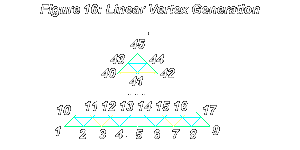 Linear tesselation is good if you are only going to use one level-of-detail for tesselating triangles. Otherwise the fractal tesselation produces a better structure, since you can dynamically cache the vertices you've already generated, and if you come closer to an object and want more detail, all you have to do is allocate space for another n(n+1)/2*3 created during the nth split. And, you can use the cached vertices to calculate the new child vertices. But linear tesselation might be good for some rasterizers because of the way it organizes the vertices. |
Triangle Strips
 |
|
We can optimize the geometry processing pipeline if we can create vertices
in memory in such a way as to form triangle strips. Then when we want to
draw the tesselated triangle we can just send several triangle strips, instead
of sending each small triangle. If they vertices are laid out in memory the
proper way, we can just send a pointer to the first vertex and the number
of vertices in the strip, and everything will be quickly processed. Sending strips requires less data than sending triangles, when the vertices are shared between triangles. We can specify n triangles using a triangle strip consisting of n+2 vertices, instead of 3n vertices that would be sent if we were sending each triangle individually. At first glance, it might seem we can form a triangle strip thus: 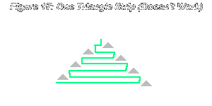 However, this isn't a triangle strip. When go to a triangle on the next level, we are using the wrong edge to connect. Actually, we'll need to begin and end several triangle strips: 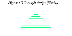 Ideally, we'd like to to have an algorithm that generates vertices in such an order that we can send a single triangle strip just by sending a pointer to the first vertex in the strip. There is no algorithm to do this directly, and if you try numbering the vertices you'll see why. Instead, we'll have to take the output from either the fractal or the linear tesselation and make it into triangle strips to send to the rasterizer. The linear tesselation method produces output which is much better suited to this task. That's because the vertices are almost in the exact order we need. For example, if we were to send figure 16 as triangle strips, the first triangle strip would consist of vertices 1 10 2 11 3 12 4 13 5 14 6 15 7 16 8 17 9. We keep alternating between the rows. In fact, if we used the linear tesselation method and in the output made every vertex be followed by an empty vertex to be filled later, all we'd have to do is copy over, from the row on the top, into the empty spaces of the row below it. Then we'd have the complete data for a triangle strip. This method would be fast and in the end we'd just send a pointer to the first vertex, and a count. For example, if we again looked at figure 16, we could use the linear tesselation method as follows: Produce the following memory structure using linear tesselation: Vtx1 ___ Vtx2 ___ Vtx3 ___ Vtx4 ___ Vtx5 ___ Vtx6 ___ Vtx7 ___ Vtx8 ___ Vtx9 ___ Vtx10 ___ Vtx11 ___ Vtx12 ___ Vtx13 ___ Vtx14 ___ Vtx15 ___ Vtx16 ___ Vtx17 ___ ... After we've tesselated, we copy the second row from the bottom into the empty spaces of the bottom row: Vtx1 Vtx10 Vtx2 Vtx11 Vtx3 Vtx12 Vtx4 Vtx13 Vtx5 Vtx14 Vtx6 Vtx15 Vtx7 Vtx16 Vtx8 Vtx17 Vtx9 ___ Vtx10 ___ Vtx11 ___ ... We repeat: copy the third row into the empty spaces of the second row, the fourth row into the third row, etc. until we reach the top row. Then we have the triangle strips ready to be sent to the rasterizer. Alright, so basically, that is how you would tesselate curved surfaces for drawing. Fractal tesselation is better for dynamic Level-Of-Detail caching. Linear tesselation is better for generating triangle strips and sending them all at once to a geometry processor. Both have their advantages, and it all depends on what your priorities are. |
But Wait, There's More!
 |
|
We are not finished. here are several more issues we should discuss, and
you've probably had enough for now. Think about what we've seen sofar, and
about how you could apply something like this in your own code. After all,
it's Theory To You until you put it into practice. So stay tuned until the
next issue, when the rest will be revealed! Until then, feel free to send me some email. Also, you might want to check out these links: |
Links And Acknowledgements
 |
|
Thanks to Eric Hawkes from Stanford for his excellent overview of
Bezier curve mathematics, and the Java applet to which I link. If you thought my overview of Bezier surfaces was too skimpy, you'd can read a much more complete tutorial on them. Read a paper by Haim Barad, which talks about "Tesselation of 4x4 Bezier Patches for the Intel III Processor." I will provide more links when I finish up the discussion in the next installment :) |