|
A Small, Portable 3D Engine by (21 August 2001) |
Return to The Archives |
Introduction
 |
|
For the last few years at school, I’ve been using a TI-85 Graphing calculator. About a year and half ago, I tried to write a simple orthographic display, but it never got anywhere. Last month, I was extremely bored in math class, so I decided to see what I could program. I suddenly came up with a great idea for a perspective projection and implemented it. Various enhancements and optimizations have led to the 3D engine I use today. This article will describe the evolution of my engine from a sample program to a full library of portable software rendering functions, and document this library, called pGL (portable GL). The library interface is based on OpenGL (as much as a set of TI-85 programs can be based on C), because it is very simple and easy to use, and I also don’t need to replicate the long initialization and error-checking routines of DirectX. This library was written on a TI-85, but it should be very easy to port to other devices, including full computers. The TI-85 is extremely slow and only has 28KB of built-in memory, so there is no way to get a real-time engine in there without using one of the TI-series assembly programming kits around, which I do not have. However, on a more powerful device (I would like to port it to my Nomad Jukebox, since it has sufficient power, but that’s not exactly possible), it should be easy to run in real-time. I wrote the rendering code with a very simple algorithm, and the only matrix math is in the tranlate, scale, and rotate functions, so it should be very simple to understand. This is an easy algorithm to use (although it does make it hard to do mass rasterization, as it uses operations that can’t be applied to an entire matrix in one operation), and should work well on any programmable device with a screen. |
|
Requirements
|
|
The engine has several requirements. It was originally developed on a TI-85, which has many built-in math functions, so these functions (such as matrix and vector math) will not be described here. However, there is an advantage to implementing these yourself: you can optimize them specifically for the engine, and make them intentionally break the rules to allow faster data processing. The engine can run on any programmable processor with enough memory to store the code and a suitable output device. I run it on my TI-85, which is too slow for real-time rendering, but on more advanced deviced such as a PDA (or anything better than a graphing calculator) it should be possible to run at least simple renderings in real-time. If you are running in an environment with limited memory, it is probably best to generate the data at render-time if possible, as I will describe in the section about the sphere model I added. If you have lots of memory, it would be interesting to experiment with stored models. |
|
History
|
|
My first idea for software rendering was implemented in a small test program that displayed the corners of a cube (once I got it to work). This was a while ago, so I can’t remember the (potentially useful) solutions to the problems I encountered, but I’ll try to give an accurate history of the development of the engine. Back to the rendering process: I decided that the renderer would use a fixed point of view looking up the z axis (in the positive z direction, the opposite of OpenGL). The point of view would be at a position around (0,0,–20). A screen would be defined to exist at (0,0,0), with the height and width set in variables (see Figure 1). 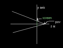 To transform a point to screen space, I started by finding the vector from the point to the viewpoint, vpv. I then found the distance from the viewpoint to the screen (vsd), and from the viewpoint to the point (vpd). By finding vsd/vsd and multiplying that by vpv, I found the vector from the viewpoint to the location where the point is projected on the screen. I then found the distance from the top and right sides of the screen to this intersection point, divided them by the screen size in world-space (the co-ordinate space all points are in), and multiplied them by screen size in screen-space (the co-ordinate space of the screen) to give me the location of the point. I then used the TI-85’s PointOn function to display the point. Those of you familiar with TI graphing calculator programming will know that choosing a point location isn’t as easy as specifying the pixel offset from the top-left corner on the 128x64 screen. The screen co-ordinates are actually defined in the same co-ordinate space that is used for graphing. I run the engine with the x range being –10 to 10 and the y range being –5 to 5, to have a correct unit-to-pixel ratio in each direction. This is not a problem when you get used to it, but if you want to implement this on another device, you should be aware of how screen co-ordinates are handled in this document. This method was very inefficient, because it took many steps to compute the screen location, and I had to have an actual screen in the world-space that was separated from the viewpoint, if only by a small distance. My next revision of the algorithm worked much better. I soon found a much more efficient way to compute the position: I calculated the parameters to have a screen at the z position of the vertex, and did my old transformation in place. It’s best explained with a picture, so take a look at Figure 2. The point in this example is 50 z units away from the viewpoint (which is now at the origin). By calculating that it’s 30 units down from the top, with a total height at that z position of 100 units (unlike my drawing, the view frustrum is symmetrical). That means that the point is offset from the top of the screen by 30% of the height. I do the same thing to find the x co-ordinate. 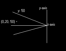 Finding the height and width of the frustrum for any z position is the most important part of this algorithm, and fortunately it’s very easy. We’ll start by imagining a triangle consisting of the z axis cut off at the origin and the z co-ordinate we want (segment Z), a line extending from (0,0,z) to the height at that position (segment V), and the hypotenuse (segment H), which we will ignore (see Figure 3). 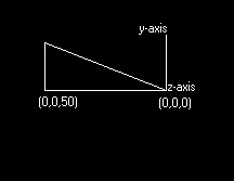 We know that the angle between the z-axis and the hypotenuse is ˝ of the field of vision (45° in my engine), because there is another inverted but identical triangle before this one, and they share the field of vision. I store the half-field-of-vision on a variable we’ll call hfov. I use the tangent for this because we know that So up to now, here’s how the algorithm works: for each vertex, where Z is the distance from the point of view to the vertex, we do To summarize the transformation operation, here’s the two formulas, where sw is the screen width, sh is the screen height, fw is the frustrum width at that point, fh is the frustrum height at that position, p is the point, and the point of view is at (0,0,0) (if not, simply change p to be p – pov): While developing the vertex transformations, I had kept the transform code in a separate program called glVertex. Because of the limitations of the TI-85, I had to create this function as a separate program, and then pass the data in a predefined vector called p. The program operated on this to display a point on the screen. It’s about this time that I probably implemented the translation and scaling functions. Once again taking OpenGL-like names, I named the matrix that each vertex would be multiplied by as glMdlv. The translation matrix is easy to use. Where translation is tx, ty, and tz, the matrix is defined as this: 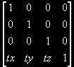 .
The scaling matrix, where sx, sy, and sz define the scaling, is .
The scaling matrix, where sx, sy, and sz define the scaling, is
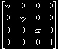 .
When translating, I add the translation to the relevant values, and
when scaling I multiply the relevant values by the scaling (so if you
scaled each dimension by 2 then by .5, you’ll end up with normal
scale). To understand how these matrices work, you really need to
understand vector multiplication, but here’s an example of how
the translation and scaling matrix put together work, with a vector
vertex of [10,20,30,1]: x = sx*10 + 0*20 + 0*30 + 1*tx, y = 0*10 +
sy*20 + 0*30 + 1*ty, z = 0*10 + 0*20 + sz*30 + tz*1, and w (the 1) =
0*10 + 0*20 + 0*30 + 1*1. This means that x = 10sz+tx, y = 20sy+ty,
and z = 30sz+tz. This is how matrices are applied to vectors to
transform them. The rotation is done through the same matrix, but
it’s more complex and I’ll cover it later. .
When translating, I add the translation to the relevant values, and
when scaling I multiply the relevant values by the scaling (so if you
scaled each dimension by 2 then by .5, you’ll end up with normal
scale). To understand how these matrices work, you really need to
understand vector multiplication, but here’s an example of how
the translation and scaling matrix put together work, with a vector
vertex of [10,20,30,1]: x = sx*10 + 0*20 + 0*30 + 1*tx, y = 0*10 +
sy*20 + 0*30 + 1*ty, z = 0*10 + 0*20 + sz*30 + tz*1, and w (the 1) =
0*10 + 0*20 + 0*30 + 1*1. This means that x = 10sz+tx, y = 20sy+ty,
and z = 30sz+tz. This is how matrices are applied to vectors to
transform them. The rotation is done through the same matrix, but
it’s more complex and I’ll cover it later.To initialize the modelview matrix (glMdlv) and the environment, I wrote a program called glInit. I added a little logo to look at while it works (about 5 seconds on my TI-85), that I’ve reproduced in the code section in the 8x21 format of the TI-85 screen in case you want to throw it in (note that on a TI graphing calculator you need to use one command to display each line) After this I added scaling first, with a program called glScale, which took a 3-member vector called scl and multiplied each element by the corresponding element in the modelview matrix. The next program I added was glTranslate, which again used a vector named scl and added it to the corresponding elements in the modelview matrix. Around this time, I decided to add a function for making full polygons. I modified the glVertex program to work in three modes: GL_QUADS, GL_TRIANGLES, and GL_POINTS. These modes were set and initialized by a program called glBegin, and the mode was stored in glMode. In every mode I would transform vertices as soon as they came in. In GL_POINTS mode I displayed them immediately, but in the other two modes I accumulated them until I had enough to draw the full polygon using the built-in Line function. Once I had all this implemented, I made a program that used the functions to display a cube (see Listing 1.1). After successfully scaling and translating the cube with temporary control interfaces, I decided to add the rotation. The rotation was the longest part of development, as I went through several generations of code and finally back to my original solution, trying to get around problems. In the start, I found a document that described x, y, and z rotation matrices and implemented these in a function called glRotate. It screwed up at first because I used normal rotation matrices for angles of 0°, when they should have been identity matrices. This didn’t work because I multiplied the matrices directly with glMdlv. I also probably multiplied in the wrong order, so even the correct operations didn’t work. I then tried moving the rotations to a separate matrix, where I would add the rotation matrices. This, of course, did not work either. Since nothing was working, I changed the architecture of the transformation functions. I decided that the translation, scaling, and rotation would be stored in three vectors, and every time I did a transform operation, these would be updated before calling the program glBuildMatrix to generate glMdlv and three rotation matrices from scratch. When transforming a vertex, I would simply multiply it by glMdlv, glXRot, glYRot, and glZRot. This did work, but I soon began to wonder why (vertex)*(glMdlv)*(glXRot) would not be the same as (vertex)*(glMdlv*glXRot). I tried this associativity inside the transformation function and it worked, so I decided to move back to incremental operations inside the transformation functions. I restored the glScale and glTranslate functions to their previous state, but the rotation function took a bit of experimentation to succeed. After some experimentation, I came up with this solution: for each rotation matrix (x, y, and z), if the rotation for that axe was non-zero, I would build the matrix assign glMdlv*(rotation matrix) to glMdlv. I will go into more detail about this in the listing for the glRotate function. Sometime between my first attempts at rotation and my final version, I separated and enhanced the transformation and rendering process. I move the transformation component into a new function that could operate on a matrix containing a number of vertices, and then transform them into screen space individually and store these co-ordinates in another matrix. It ended up as three functions: glTfrm, glVertex, and glVtxs. The glTfrm function did transforms, by first applying the glMdlv matrix and then moving vertices to screenspace. It had two modes: single vertex and vertex array. To operate in single vertex mode, tfMode had to be set to 1, and the function was called from glVertex, which is called by a program to display or queue a vertex. If tfMode was not 1, the function operated in vertex array mode. In this mode it was called by the program doing the rendering instead of glVertex, and it stored all the resulting screen co-ordinates in a matrix. When a program is operating in vertex array mode, it has to do four steps: 1) set the correct vertex mode (quads, triangles, or points), 2) load the vertices into a matrix and set the number of vertices in nVerts, 3) call glTfrm, and 4) call glVtxs. A non-vertex array program only has 3 steps: 1) set the vertex mode, 2) load the vertices one at a time into the p vector, and 3) call the glVertex function for each vertex. I don’t remember the exact reasons it ended up this way, but the end result was that using a vertex array involved calling glTfrm to generate the screen co-ordinates and then called glVtxs to actually display the model. At this point I was still using my cube model from the beginning. Once I was done with the pGL library, I started to play with the program that displays the model. I set up a main loop where it would render the model, pause, and go to the control screen. The control screen does x and y rotations and translations (see Figure 4). I added a “scale” variable that set the change to the rotation or location at each keypress, so it could be moved 100 units or .1 units. I might move this control screen into another program to be able to use it from new programs. After I was done with the cube program, I made a sphere and several other models before I had to return my calculator (I cleaned up the internal organization a bit first) |
|
Functions
|
|
Here are the function listings, in pseudo-TI-85 code. This modular library should be easy to port to any device (if I had a PDA it would be on there by now). I don’t include texturing, shading, or filling, as I couldn’t do anything that processor-intensive, but if you add those you’ll have a simple software renderer, similar to the original Quake. This could also be used as the base for the development of a full PC-based game engine - there’s only a few rendering functions missing. Comments in the code will be in C++ style - if you are using this on a TI calculator, remember not to put in the comments, as it doesn’t recognize comments. If you are putting this on a TI-85 calculator, remember to change ‘a=b’ to ‘b->a’ for assignments. Matrices and vectors are in brackets. I recommend that you read the entire source, as I have comments on the concepts and presentation involved that I don’t repeat, and you may need them to understand what the code actually does.
The aspect ratio is based on physical measurements. The pixel ratio is already factored in, so with an ar of 1 a unit of width would be twice as many pixels as a unit of height (128x64). You could add the pixel ratio to this aspect ratio. The end result should be that 1 vertical unit has the same physical length as one horizontal unit. On the TI-85 the screen co-ordinates are set as the x and y range for graphing (xMax, xMin, yMax, yMin), and then you use those graphing co-ordinates to draw the pixels, so I set the above-mentioned variables to 10, -10, 5, and -5 respectively. If you are using pixel co-ordinates, you will already have the pixel aspect ration incorporated and you just need to use the physical aspect ratio - I had to do this to get consistent screen-co-ordinate to pixel ratios. This adjustment is done outside of the program, so if you use a TI calculator, or one with the same display system, you will have to do it to use the engine properly.
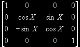
If X // the order is important here. If you reverse these, it will not work correctly
|
 * glMdlv
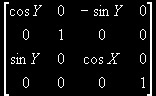 * glMdlv
If Z
glMdlv =
* glMdlv
If Z
glMdlv = 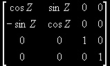 * glMdlv
|
Conclusion
|
| The design and implementation of this library was interesting and helped pass many boring math and physics classes (boring as in ‘I already did this 5 years ago, why do I have to be taught it again by teachers who know less than me (at least in nuclear physics)’). I’d like to know how far it would go, as I don’t have a PDA to try it on and I have bigger projects on my computer - I also haven’t figured out how to reverse-engineer my MP3 player to get some visualizations running on the screen ;). Some of these concepts are thanks to Lionel Brits’ Matrices: An introduction, where I learned a lot about matrices and the transform, scaling, and rotation matrices. It’s a great page for learning more about matrices. Now, go forth and port! |
|
|