|
3D Graphics on Mobile Devices - Part 2: Fixed Point Math by (16 August 2003) |
Return to The Archives |
Introduction
 |
| This is the second part of the series of articles on 3D graphics for mobile devices. In the first article I described the Symbian platform and its limitations, and some technical details about a voxel engine implementation. In this article I will discuss fixed point mathematics, in preparation of the third and fourth article, which will describe a 3D engine that I am developing for Overloaded, which will be used for a 3D race game currently under development. |
|
Racing Game
|
 After the development of the game 'Resistance' we wanted to do a racing game. Resistance is a huge hit, when it comes to convincing partners that we produce the most advanced technology for mobile games. That's nice of course, but we wanted to do something that also appeals to our customers. A racing game is perfect for that. Its a genre that benefits greatly from advanced technology like 3D graphics, physics and AI while at the same time even inexperienced players like to drive a car around.
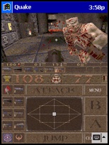
We found the voxel engine to be slightly limiting for a racing game. The landscape texture is a bit coarse (or the track becomes too small), you can't have vertical polygons, and camera movement is limited which is a pity when you want cool replays. So we decided to build another engine: A basic polygon engine. For mobile devices, you can't just grab some free 3D engine source code and adjust it for the smaller screen, because the ARM processor does not have a floating point unit. Floating point instructions can be used, but they are emulated, at rougly 5% of the speed of integer calculations. Someone ported Quake to the PocketPC (which uses a 200Mhz StrongARM processor), and it runs at 5-12 fps. Quake runs fine on a P90, so you would expect excellent performance on a 200Mhz device. Excellent performance is possible, but not without modifying the engine at it's heart: All math must be done in fixed point. |
|
Fixed Point Math
|
|
I'll briefly summarize how fixed point math works. If you're familiar with the concept, just skip to the next paragraph. Suppose you want three decimal digits, but you don't want to use floating point. You could do this by multiplying all numbers by 1000. As long as you don't forget to divide the result of your calculations by 1000, you can do all your math this way. Adding 1.3 and 2.6 for example: 1300 + 2600 = 3700 (I'll leave it as an excercise for the reader to spot the error in this equation). Multiplication is slightly trickier: 1500 * 1000 = 1500000, and as you can see, the result of the multiplication is a factor 1000 too large, so you'll have to compensate for that. Division works the other way round: 1500 / 1000 = 1 (int!), so you should have multiplied one of the numbers by 1000 before doing the division. Now exchange the '1000' figure with a random power of two (like 1024), and you have something that can be used conveniently and fast. Converting to and from fixed point becomes a matter of shifting, just like compensating for large numbers after multiplication. So much for the basics. There's plenty of basic info on fixed point maths on the web, so if you need more, use google. :) |
|
Range and Precision
|
|
The basics are simple, but actually using fixed point maths to do an entire 3D engine is less trivial. A 3D engine needs accurate maths all over the place: For transformation, projection and rasterization. For my 3D engine, I developed a set of classes that handles the basics of 3D maths, at a decent accuracy and a predictable range. Let's define 'decent accuracy' first: Ideally, you would want an cummulative error that is small enough not to affect the positioning or coloring of any pixel of the final rendered image. Let's consider a simple example of this. Suppose you are writing a full-screen zoom effect. When drawing a scanline, you will be interpolating from a U coordinate (U1) to another U coordinate (U2) when sampling the source texture. Suppose the scanline is 256 pixels. Then, for each pixel drawn we will add (U2 - U1) / 256 to a variable that holds the current U position. Let's call this stepsize 'delta_u'. How accuracte needs delta_u to be? This can be determined as follows: As long as the cummulative error does not exceed one, truncating it will give the same result as a perfectly accurate calculation. We are interpolating in 256 steps, so each step, the error may not exceed 1/256th. The error that each step could theoretically add is the magnitude of the first bit that we are not storing in delta_u. Suppose we used 8 bits for the fractional part. In that case, we are not storing the 9th bit, so the maximum error is 1/512th. This means that we could have used 7 bits of fractional precision to do this interpolation. In the above example, if we would have used the minimum fractional accuracy, we would have used 7 bits for the fractional part, which leaves 31 - 7 for the integer part (or 32 - 7, since we can probably omit the sign in this case). This leaves 25 bits for the integer part. This means that our zoomer will never be able to use a texture that is wider than (1 << 25) pixels. This is probably not a problem, but it does show the direct link between accuracy and range. Let's apply this to some vector maths. Suppose we have a transformation / translation matrix. The matrix probably consists of three nicely normalized vectors plus a translational part. We thus know that the transformation part does not need to hold any numbers outside the range -1..1, wich means that two bits should suffice for the integer part. This leaves 30 bits for the fractional part, which is great, especially when we are concatenating lots of these matrices. The translational part on the other hand determines the size of our world, so we are not going to accept two bits of integer accuracy here. |
|
Reality
|
Let's see how this works in real life. First, we define a couple of convenient macro's:
I'm working with 16:16 fixed point numbers by default (16 integer, 16 fractional bits). I'll be converting from and to 16:16 fixed point; to convert to 16:16 fixed point I'll need to multiply by 65536, to get back to regular ints (32:0), I'll need to do a binary shift right by 16 bits. Adding and subtracting 16:16 numbers is not any different than adding and subtracting ints, but multiplying and dividing is, therefore we need another couple of macros to make those operations easier:
Since multiplying a 16:16 number by another one could result in a 32:32 number (just like 1000 * 1000 = 1 million), we need to make the neccessary arrangements to keep the ranges within limits. By pre-shifting both parameters by 6, we reduce the intermediate result to 32:20. This still doesn't fit, so using this macro limits us to multiplying 6:16 numbers without risking overflows: 6:16 * 6:16, preshifting by 6 ==> 6:10 * 6:10 ==> 12:20, exactly 32 bits. Since multiplications of two 16:16 numbers gives results that are a factor 65536 too large, we need to shift another 4 bits to get the final result. Note that the FPMUL macro can be used for larger numbers when you already know that one of the parameters is sufficiently small to compensate for the other. The FPDIV macro does something similar: Dividing 16:16 by 16:16 results in answers that are a factor 65536 too small, so essentially the result is 0:16. The macro compensates for this by preshifting the first parameter by 6 to make it larger, and the second by 6 to make it smaller. Using the macro's will make the FP math code more readable, but never forget that they are just 'convenient'. Consider the following line:
Here, 'a' and 'b' apparently used different levels of fractional precision, so 'a' is adjusted before the multiplication is performed. Hopefully the compiler gets rid of the double shift that is introduced... It's easy to overlook optimization opportunities and 'precision leaks' when using macro's without thinking over their exact workings. |
|
Vector Math
|
|
Next we need some decent vector math classes using these concepts. Here's a basic vector class declaration:
Pretty straightforward. Notice that the vector is using three integers. Instantiating the vector, adding and subtracting another vector are not any different from your regular float vector implementation. Scaling a vector (the '*' operator) uses the FPMUL macro to get some range. Next up is a matrix class:
Again, nothing special. Remarkably simple, in fact. There are some differences this time with a floating point matrix class implementation though: The identity matrix looks different:
But the interesting part is the concatenation code. I store my matrices as 4x4 matrices (transformation and translation), but I want to exploit the knowledge about the range of transformation part (3x3). So instead of using the FPMUL macro, which wastes 6 valuable bits of precision before doing the multiplication, the code below performs more accurate multiplications, except for the translational column:
Initializing the matrix to be used for rotations about the x, y and z axii is of course done using a look-up table for sinus and cosinus. I use 4096 steps for a full circle, which is accurate enough in practice.
Notice the odd passing of the precalculated sinus and cosinus tables: This is neccessary as the Symbian OS does not allow static member variables. I can't put pointers to these tables in the matrix class. Besides these classes, I implemented a plane class, a bounding sphere class and a basic frustum class. Here are links to the source files (article_mobile3d_math.cpp & article_mobile3d_math.h). These can be used in your own projects with minimal modifications. |
|
Conclusion
|
|
Using fixed point math is a neccessity on some platforms and in some cases. Its use is not limited to obscure OSes like Symbian, it can also be useful for improving performance on machines that do have a floating point unit. A Pentium is able to do calculations using the integer and floating point units simultaneously; interleaving instructions this way can dramatically speed up your code. I hope this article demistified fixed point math a bit. I also hope I showed that you can get excellent and predictable precision from fixed point math, as it seems that 3D engines on mobile devices have major problems delivering stable 3D graphics. It's possible to get perfectly stable polygons with subpixel and subtexel accuracy, I can tell you. It just takes a bit of tweaking. At the end of the next article I will show a working demo of a fixed point 3D engine. Until then - Have fun. - Jacco Bikker - a.k.a. "The Phantom" |
|
Article Series:
|